This week coincides with the third episode of our citizen science adventure on Hive. We have up to now first dealt with the installation of the MG5aMC software, which allows for computer simulations of particle collisions such as those ongoing at CERN’s Large Hadron Collider (the LHC). Then, we have moved on with a tutorial on the manner to use this program, which allowed us to simulate collisions describing the production of a pair of top-antitop quarks at the LHC. This is what we consider as our “toy signal” for the moment.
The current blog is dedicated to the natural next step: analysing this toy signal and its properties. This requires the installation of a new piece of software called MadAnalysis5 and some of its optional dependencies. Moreover, we plan to additionally use this package to investigate a bit what lies in our top-antitop signal. A full study is left for the upcoming episode, in two weeks from now.
Before dealing with the tasks of this week, I would like to shed some light on the 15 contributions to the project emerging from Hive community members, and on the amazing reports about their work that have been shared on chain.
- Episode 1 (getting started): We got seven reports from agreste, eniolw, gentleshaid, mengene, metabs, servelle and travelingmercies. The work of @metabs is in particular an excellent documentation on how to get started with a Windows system through a virtual machine.
- Episode 2 (top-antitop production at the LHC): We got eight reports from agreste, eniolw, gentleshaid, isnochys, mengene, metabs, servelle and travelingmercies.
Following the particle physics tradition, the lists above are alphabetically ordered. If you are a newcomer to this project and are interested in joining us, it is never too late to start from the beginning and move forward. Each episode is expected to take a few hours of your time, not more, and we are eagerly looking forward to reports about your work (to be posted with the #citizenscience tag).
Before moving on, I acknowledge all participants to this project and supporters from our community: @agmoore, @agreste, @aiovo, @alexanderalexis, @amestyj, @darlingtonoperez, @eniolw, @firstborn.pob, @gentleshaid, @isnochys, @ivarbjorn, @linlove, @mengene, @mintrawa, @robotics101, @servelle, @travelingmercies and @yaziris. Please let me know if you want to be added or removed from this list.
[Credits: geralt (Pixabay)]
Getting started with MadAnalysis 5 - task 1
In the previous episode, we simulated 10,000 proton-proton collisions such as those on-going at the LHC. In our simulation setup, we enforced that a pair of well-defined particles were produced, one top quark and one top antiquark. We obtained an output file with simulated collisions, tag_1_pythia8_events.hepmc.gz, that weighted about 800-900 MB.
Such a huge size is related to all phenomena occurring in high-energy particle collisions. These include the decay of all produced heavy objects, radiation by virtue of the strong interaction (one of the three fundamental forces) and hadronisation processes (the formation of composite subatomic particles made of quarks and antiquarks). For more information, you may consider checking out this older post, or even this one.
A 800-900 MB file is not something practical to use for a study. Even if information is encoded in a text-based format, it is very unpractical for any purpose. You can convince yourself by unpacking the file (executing tar xf tag_1_pythia8_events.hepmc.gz in the folder where the file is located) and by checking out its content (assuming your computer is good enough to open a 900 MB text file). However, you don’t have to absolutely do this.
From the properties of this file, we know in advance that the 900MB messy picture can be compactified by using reconstructed higher-level objects. This was detailed in this recent blog, in which I have also covered detector simulations.
This is what we will do today.
In order to allow for the simulation of particle physics detectors such as those of the LHC, we plan to use the MadAnalysis5 software. This program moreover allows us to reconstruct the final state of a simulated collision.
This means that we can start from the heavy 900MB file with the entire information, and then replace the hundreds of produced particles by a small number of higher-level objects like electrons, muons, jets, photons and missing energy. I recall that a jet is an object containing a collimated set of dozens (or sometimes even hundreds) of strongly-interacting particles (see here for more information).
The MadAnalysis5 program is available from GitHub and can be obtained by opening a fresh terminal and typing:
git clone https://github.com/MadAnalysis/madanalysis5
From there, the code can be immediately used (on some systems, you may need the python-is-python3 package to be installed). Still in the shell, we can enter the madanalysis5 directory downloaded from GitHub, and start the program.
cd madanalysis5
./bin/ma5
Following the indications printed to the screen (please answer yes to any question raised by the code), we can see that the program checks whether all mandatory dependencies are available.
This is illustrated in the picture below. In my case, I had to disable a few features that are available system-wise (those concern common particle physics software), and that should not be present on your system (as none of the participants of this citizen science project is a common user of high-energy physics tools). They should therefore be marked as disabled in your case, instead of disabled by the user as in my case. Don’t worry, this detail is irrelevant for the following.
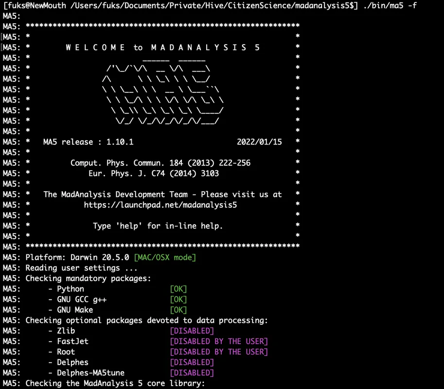
[Credits: @lemouth]
From there, MadAnalysis5 takes care of compiling its C++ core. As we installed the C++ package Pythia8 a month ago, all compilers should be up-to-date and this step should work out of the box. After 3 tests and 2 compilation steps, you should get something similar to what is displayed in the image below.
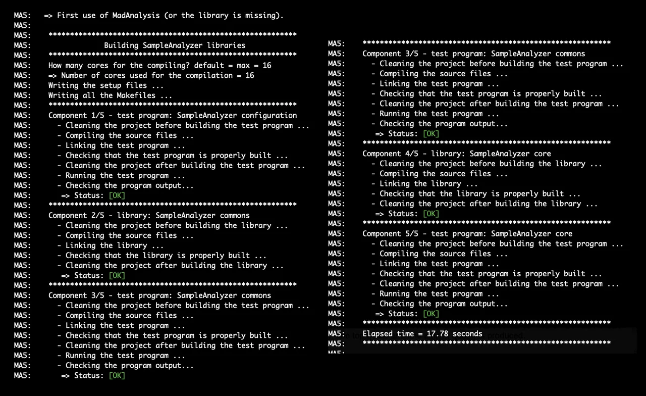
[Credits: @lemouth]
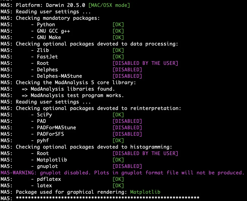
Finally, the code takes care of checking the external dependencies that are available. In my case, I obtained the following.
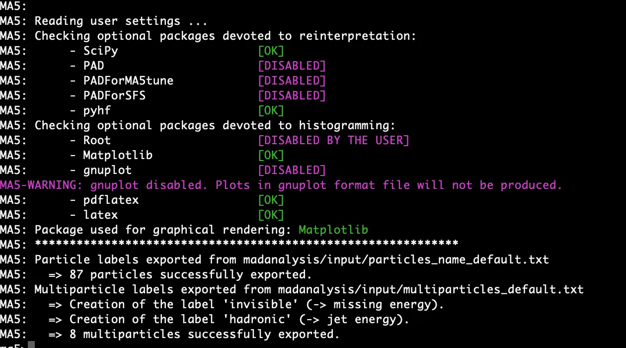
[Credits: @lemouth]
What is crucial is that the Matplotlib package is available, as well as the latex and pdflatex compilers. If this is not the case, please exit MadAnalysis5 (by typing exit in the program’s command line interface) and install those packages. Information on matplotlib is available here, and on the (pdf)latex compilers there (texlive needs to be installed).
When everything is done and went fine, you should see a prompt ma5> that is waiting for instructions.
Additional packages - task 2
We now need to update our installation of MadAnalysis5 so that it could use FastJet (event reconstruction) and zlib (reading and writing compressed event files). This is fully automated and proceeds as follows.
ma5>install zlib
After a successful installation of zlib (again, please answer yes to any question raised by the code), MadAnalysis5 needs to be restarted.
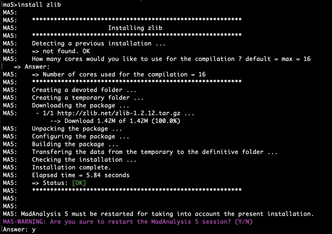
[Credits: @lemouth]
This time, the compilation of the MA5 core is more complex, and requires 4 tests and 3 compilations. The installation of FastJet is similar and is achieved by typing in the MadAnalysis5 command line interface:
ma5>install fastjet
It takes a bit more time, and the code needs to be restarted at the end of the process. The core is recompiled a last time, and we are good to go with some physics. In the following, I keep the physics part minimal. The reason is simple. If the above tasks are not straightforward, they may take some time, with the risk of having one or the other participants overwhelmed by work. Let’s avoid this!
[Credits: @lemouth]
Top-antitop simulations - task 3
In order to do some physics, we make use of the top-antitop simulations of two weeks ago. The generated event file should be located at
<MG5aMC-installation-folder>/<some-name>/Events/run_02_decayed_1/tag_1_pythia8_events.hepmc.gz
The first part of the path is the absolute path to the MG5aMC installation, and the second one is that chosen two weeks ago when casting the output command in MG5aMC. Note that the run number (02 in my case) may be different in yours. What is important is to get the full path to the generated events. Please copy paster it for later use.
Then, those events have to be imported in MA5 (I call MadAnalysis5 with the abbreviation MA5 from now on), so that we could add effects related to a typical LHC detector. In our simulations, the following detector effects are included.
- Reconstruction: Any particle that interacts with the detector material leaves into it tracks and energy deposits that need to be converted into high-level objects (electrons, muons, photons, jets). This task is not always perfect, and this is accounted for through reconstruction efficiencies.
- Smearing: The resolution of the detector slightly degrades the estimation of any particle property. Some quantities are thus smeared (their value is modified according to some Gaussian law).
- Identification: An object of type A can always be mis-identified as an object of class B with some probability.
After the simulation of the detector, MA5 reconstructs higher-level objects, and store the output in a fresh event file. In this file, each event contains a small number of electrons, muons, jets, photons and missing energy.
In practice, everything detailed above is done as follow. First, MA5 has to be started as
./bin/ma5 -R madanalysis/input/ATLAS_default.ma5
This instructs the program that a detector simulation has to be used when event reconstruction is at stake (the program will print a lot of things to the screen; if interested on what this is, feel free to ask questions as comments to this post). Moreover, we tell the program that the detector has the characteristics of the ATLAS detector of the LHC (this was a random choice).
Second, we need to import our events and indicate the name of the output file (I choose the super original name myevents.lhe.gz).
import <path-to-our-events>
set main.outputfile = myevents.lhe.gz
submit
The <path-to-our-events> is the path to tag_1_pythia8_events.hepmc.gz mentioned at the beginning of this section.
From there, we let the code run… It may take some time…
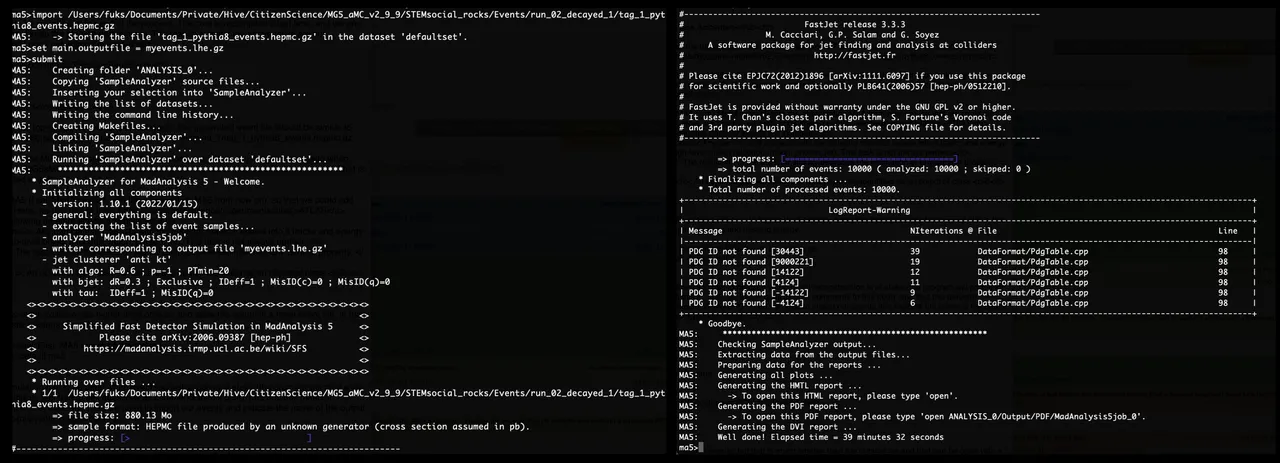
[Credits: @lemouth]
When the run is over, we can exit the program (by typing exit). We obtain a file containing 10,000 events, but that is much smaller in size than the original file. Moreover, it is human-readable and can be open with a text editor. Feel free to check it out. The file is located in the folder ANALYSIS_0/Output/SAF/_defaultset/lheEvents0_0 where the index zero is incremented at each MA5 run.
The file that is there should be of about 7-8 MB, which is much more manageable that 800-900 MB. Note that this file begins with a long commented out part that explains how to read it.
Some physics - task 4
As a single physics task for today, we analyse the generated output file in order to investigate the content of the produced events in terms of electrons, muons, jets, etc. This is done by restarting MA5 normally (./bin/ma5). From there, we type the commands
ma5> import ANALYSIS_0/Output/SAF/_defaultset/lheEvents0_0/myevents.lhe.gz as ttbar
ma5> set ttbar.xsection = 505.491
ma5> plot NAPID
ma5> submit
The first line above allows us to import the generated events (myevents.lhe.gz) and to assign to them the label ttbar. The second line tells MA5 that the production cross section associated with this event sample is 505.491 pb. I recall that we computed this value during the second episode of our project. In the third line, we ask MA5 to plot a histogram displaying the particle content of the events, stacking the results of every single event. The fourth line simply indicates to MA5 that it can start the calculation.
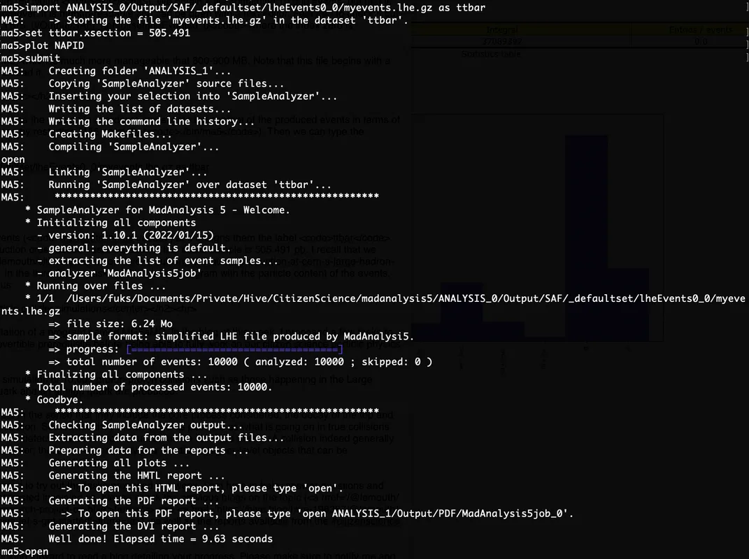
[Credits: @lemouth]
When the run is over, it is sufficient to type open to get to the results displayed in a browser. We should see a figure similar to that one:
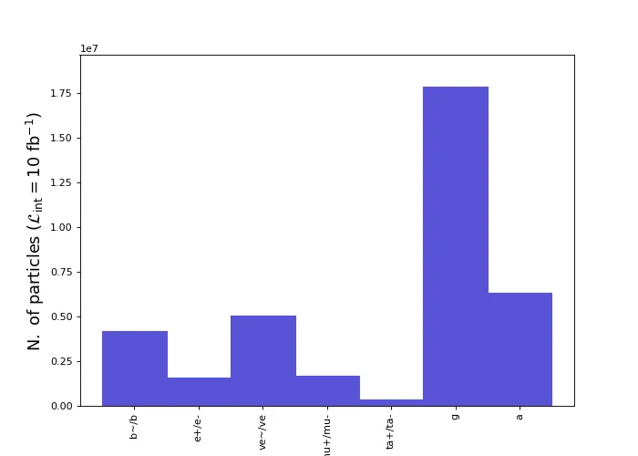
[Credits: @lemouth]
We observe that our events contain a lot of b-jets (the b/b~ column), some electrons (the e+/e- column) and some muons (the mu+/mu-~ column), very few taus (the ta+/ta- column), some missing energy (the ve/ve~ column), really a lot of jets (the g column) and a bunch of photons (the a column).
This distribution is expected from the decays of the produced top and antitop particles. Each decay gives rise to one b-jet (that is a jet of strongly-interacting particles originating from a b-quark) and a W boson. The latter can further decay into an electron and missing energy, or into a muon and missing energy, or into a tau and missing energy, or into two jets. In addition, jets and photons are additionally coming from radiation. I hope that with this short explanation, you understand why we have obtained the figure above.
If you don’t understand everything so far (in particular why we get the results we got), please don’t worry, I will come back to this in two weeks, with much more details and with an episode dedicated to physics only. What matters for now is to get to this figure.
Summary: detector simulations and reconstruction
The present episode of our citizen science project on Hive was dedicated to the installation of the MA5 software and some of its dependencies. This program allows us first to achieve the simulation of an LHC detector and add its impact on simulated collisions, and second to reconstruct the outcome of a simulated collision in terms of a small number of higher-level objects (electrons, muons, jets, etc.).
As a small physics exercise, we started from the top-antitop events generated two weeks ago and added the effects of the ATLAS detector of the LHC on them. We then reconstructed those events and investigated their content in terms of high-level objects.
I hope that everyone will have fun to participate to the tasks proposed this week, and I am looking forward to read your reports. If you are new to this and interested in joining us, again please consider starting from the beginning (see episode 1 and episode 2), write reports for each episode (so that I could discuss your findings with you), before embarking into the present third episode.
As usual, please make sure to notify me when writing a report, and to use the #citizenscience tag. Have a nice week, full of particle physics!