In this video I go over further into the wonderful world of sequences and series, and this time go over Taylor and Maclaurin series. These series are precise and ingenious ways of approximating many functions by only knowing all of the function’s derivatives at a specific value; in the case of the Maclaurin series it is as x = 0. These series can also be used to integrate functions that don’t have elementary antiderivatives and thus are utilized in many computers and calculators as the basis behind many types of calculations.
Interestingly, it was this very concept of Taylor and Maclaurin series that first gave me the idea of creating a YouTube channel to better learn and organize my learning of mathematics and beyond. Taylor and Maclaurin series, as well as infinite series in general, require the coming together of many mathematical concepts and thus I had then realized while still in University that I need to fully refine my mathematical knowledge. And this particular video is the perfect illustration of such a culmination of so many various mathematical concepts.
The topics covered in this video are listed below with their time stamps.
@ 1:14 – MES Note on Taylor and Maclaurin Series
- @ 5:16 - Introduction to Taylor and Maclaurin Series
- @ 21:38 - Theorem 1
- @ 22:41 - Taylor Series
- @ 24:43 - Maclaurin Series
- @ 26:25 - Historical Note on Taylor and Maclaurin
- @ 27:37 - Example 1
- @ 35:00 - When is a Function Equal to the Sum of Its Taylor Series?
- @ 36:18 - Taylor Polynomials
- @ 49:01 - Theorem 2
- @ 49:49 - Taylor's Inequality
- @ 51:36 - Proof for n = 1
- @ 1:14:09 - Equation 1
- @ 1:15:03 - Note on Alternatives to Taylor's Inequality
- @ 1:17:41 - Example 2: ex
- @ 1:30:11 - Historical Note on Calculating the Number e
- @ 1:31:15 - Example 3
- @ 1:35:04 - Example 4: sin x
- @ 1:48:33 - Example 5: cos x
- @ 1:55:31 - Historical Note on Maclaurin Series
- @ 1:56:23 - Example 6: x cos x
- @ 1:58:04 - Example 7
- @ 2:11:23 - Note on Power Series
- @ 2:12:30 - Comparing Taylor and Maclaurin Series
- @ 2:15:44 - Example 8: (1 + x)k
- @ 2:32:26 - The Binomial Series
- @ 2:45:43 - Example 9
- @ 2:59:09 - Table 1: Important Maclaurin Series and Their Radii of Convergence
- @ 3:04:12 - Integrating Functions that Don't Have Elementary Antiderivatives
- @ 3:09:35 - Example 10: e-x2
- @ 3:28:43 - Example 11: Evaluating Limits
- @ 3:38:26 - Multiplication and Division of Power Series
- @ 3:39:33 - Example 12
- Exercises
- @ 3:57:28 - Exercise 1: A Function Not Equal to its Maclaurin Series
- @ 4:17:05 - Exercise 2: Proof of Taylor's Inequality for n = 2
- @ 4:37:01 - Exercise 3: Proof of Binomial Series
Watch Video On:
- 3Speak:
- Odysee: https://odysee.com/@mes:8/sequences-series-Taylor-and-Maclaurin-Series:e
- BitChute:
- Rumble: https://rumble.com/v1v8brg-infinite-sequences-and-series-taylor-and-maclaurin-series.html
- DTube:
- YouTube:
Download Video Notes: https://1drv.ms/b/s!As32ynv0LoaIiIFz-mgCcPKh_6t2Sg?e=vhxEFP
View Video Notes Below!
Download These Notes: Link is in Video Description.
View These Notes as an Article: @mes
Subscribe via Email: http://mes.fm/subscribe
Donate! :) https://mes.fm/donateReuse of My Videos:
- Feel free to make use of / re-upload / monetize my videos as long as you provide a link to the original video.
Fight Back Against Censorship:
- Bookmark sites/channels/accounts and check periodically
- Remember to always archive website pages in case they get deleted/changed.
Join my private Discord Chat Room: https://mes.fm/chatroom
Check out my Reddit and Voat Math Forums:
Buy "Where Did The Towers Go?" by Dr. Judy Wood: https://mes.fm/judywoodbook
Follow along my epic video series:
- #MESScience: https://mes.fm/science-playlist
- #MESExperiments: @mes/list
- #AntiGravity: @mes/series
-- See Part 6 for my Self Appointed PhD and #MESDuality Breakthrough Concept!- #FreeEnergy: https://mes.fm/freeenergy-playlist
NOTE #1: If you don't have time to watch this whole video:
- Skip to the end for Summary and Conclusions (If Available)
- Play this video at a faster speed.
-- TOP SECRET LIFE HACK: Your brain gets used to faster speed. (#Try2xSpeed)
-- Try 4X+ Speed by Browser Extensions or Modifying Source Code.
-- Browser Extension Recommendation: https://mes.fm/videospeed-extension
-- See my tutorial to learn more: @mes/play-videos-at-faster-or-slower-speeds-on-any-website- Download and Read Notes.
- Read notes on Steemit #GetOnSteem
- Watch the video in parts.
NOTE #2: If video volume is too low at any part of the video:
- Download this Browser Extension Recommendation: https://mes.fm/volume-extension
Infinite Sequences and Series: Taylor and Maclaurin Series

MES Note on Taylor and Maclaurin Series
When I first learned of Taylor and Maclaurin series while still in university, it was the first time that I realized that I needed to figure out a way to make it easy to learn and, more importantly, retain knowledge regarding mathematics.
Although it wasn't until a few years later that I finally decided to create a YouTube channel to help myself continually learn and build upon mathematics, the initial spark that led to Math Easy Solutions was my first encounter with Taylor and Maclaurin series.
And this video comes full circle as I break down Taylor and Maclaurin series in-depth while utilizing and referencing many of my previous videos; thus effectively demonstrating why I created this channel in the first place. #LearnHowToLearn
Calculus Book Reference
Note that I mainly follow along the following calculus book:
- Calculus: Early Transcendentals Sixth Edition by James Stewart
Topics to Cover
- Introduction to Taylor and Maclaurin Series
- Theorem 1
- Taylor Series
- Maclaurin Series
- Historical Note on Taylor and Maclaurin
- Example 1
- When is a Function Equal to the Sum of Its Taylor Series?
- Taylor Polynomials
- Theorem 2
- Taylor's Inequality
- Proof for n = 1
- Equation 1
- Note on Alternatives to Taylor's Inequality
- Example 2: ex
- Historical Note on Calculating the Number e
- Example 3
- Example 4: sin x
- Example 5: cos x
- Historical Note on Maclaurin Series
- Example 6: x cos x
- Example 7
- Note on Power Series
- Comparing Taylor and Maclaurin Series
- Example 8: (1 + x)k
- The Binomial Series
- Example 9
- Table 1: Important Maclaurin Series and Their Radii of Convergence
- Integrating Functions that Don't Have Elementary Antiderivatives
- Example 10: e-x2
- Example 11: Evaluating Limits
- Multiplication and Division of Power Series
- Example 12
- Exercises
- Exercise 1: A Function Not Equal to its Maclaurin Series
- Exercise 2: Proof of Taylor's Inequality for n = 2
- Exercise 3: Proof of Binomial Series
Introduction to Taylor and Maclaurin Series
In the preceding video we were able to find power series representations for a certain restricted class of functions.
Here we investigate more general problems:
Which functions have power series representations?
How can we find such representations?
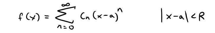
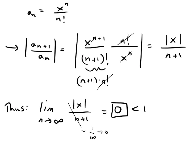
We start by supposing that f is any function that can be represented by a power series:
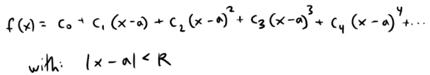
where R is the radius of convergence, and referenced below from my earlier video.
@mes/infinite-sequences-and-series-power-series
Retrieved: 19 December 2019
Archive: https://archive.ph/kAeuV

Let's try to determine what the coefficients cn must be in terms of f.
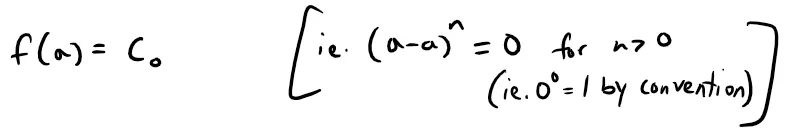
To begin, notice that if we put x = a in the above equation, then all terms after the first one are 0 and we get:
By Theorem 1 from my earlier video and shown below, we can differentiate the series in f(x) term by term:
@mes/infinite-sequences-and-series-representations-of-functions-as-power-series
Retrieved: 22 January 2020
Archive: https://archive.ph/P6xfY


Thus, differentiating f(x) term by term, we obtain:
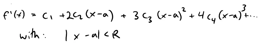
and substitution of x = a in f'(x) gives:

Now we differentiate f'(x) and obtain:
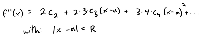
Again we put x = a in f''(x). The result is:

Let's apply the procedure one more time.
Differentiation of the f''(x) series gives:
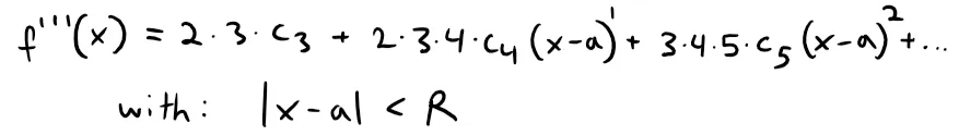
and substitution of x = a in f'''(x) gives:

By now you can see the pattern.
If we continue to differentiate and substitute x = a, we obtain:

Solving this equation for the n-th coefficient cn, we get:

This formula remains valid even for n = 0 if we adopt the conventions that 0! = 1 and f(0) = f.
Thus we have proved the following theorem.
Theorem 1
If f has a power series representation (expansion) at a, that is, if:
then its coefficients are given by the formula:

Substituting this formula for cn back into the series, we see that if f has a power series expansion at a, then it must be of the following form:
Taylor Series
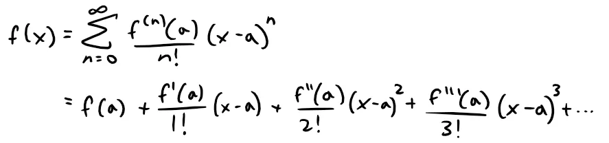
This series is called the Taylor series of the function f at a (or about a or centered at a).
For the special case a = 0 the Taylor series becomes:
Maclaurin Series
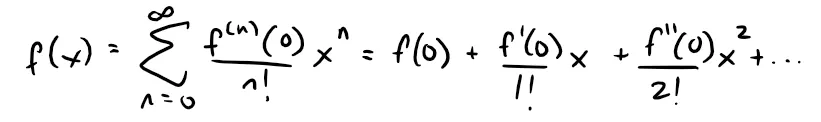
This case arises frequently enough that it is given the special name Maclaurin series.
NOTE:
We have shown that if f can be represented as a power series about a, then f is equal to the sum of its Taylor series.
But there exist functions that are not equal to the sum of their Taylor series.
An example of such a function is given in Exercise 1 at the end of this video.
Historical Note on Taylor and Maclaurin
The Taylor series is named after the English mathematician Brook Taylor (1685 - 1731) and the Maclaurin series is named in honor of the Scottish mathematician Colin Maclaurin (1698 - 1746) despite the fact that the Maclaurin series is really just a special case of the Taylor series.
But the idea of representing particular functions as sums of power series goes back to Newton, and the general Taylor series was known to the Scottish mathematician James Gregory in 1668 and to the Swiss mathematician John Bernoulli in the 1690s.
Taylor was apparently unaware of the work of Gregory and Bernoulli when he published his discoveries on series in 1715 in his book Methodus incrementorum directa et inversa.
Maclaurin series are named after Colin Maclaurin because he popularized them in his calculus textbook Treatise of Fluxions published in 1742.
Example 1
Find the Maclaurin series of the function f(x) = ex and its radius of convergence.
Solution:
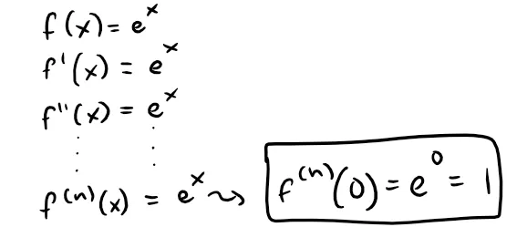
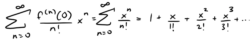
Therefore the Taylor series for f at 0 (that is, the Maclaurin series) is:
To find the radius of convergence, we can use the Ratio Test, referenced below from my earlier video.
@mes/infinite-sequences-and-series-absolute-convergence-and-the-ratio-root-tests
Retrieved: 17 September 2019
Archive: http://archive.fo/ANfgj
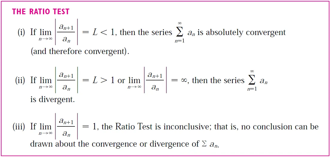
Thus we let:
So, by the Ratio Test, the series converges for all x and the radius of convergence is R = ∞.
When Is a Function Equal to the Sum of Its Taylor Series?
The conclusion we can draw from Theorem 1 and Example 1 is that if ex has a power series expansion at 0, then:

So how can we determine whether ex does have a power series representation?
Let's investigate the more general question:
Under what circumstances is a function equal to the sum of its Taylor series?
In other words, if f has derivatives of all orders, when is it true that:
As with any convergent series, this means that f(x) is the limit of the sequence of partial sums.
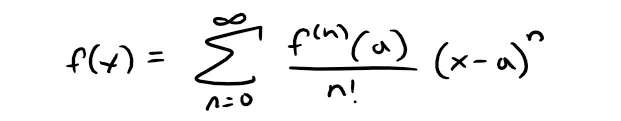
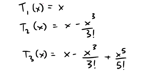
Taylor Polynomials
In the case of the Taylor series, the partial sums are:
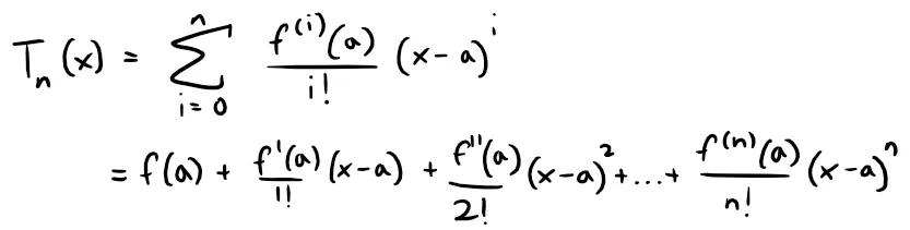
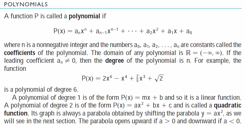
Notice that Tn is a polynomial of degree n called the n-th degree Taylor polynomial of f at a.
Polynomials and their terminology are referenced from my earlier video below.
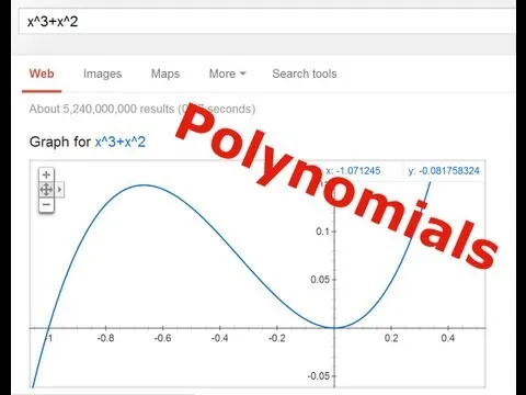
Retrieved: 17 January 2020
Archive: https://archive.ph/wip/WdFYE
For instance, for the exponential function f(x) = ex, the result of Example 1 shows that the Taylor polynomials at 0 (or Maclaurin polynomials) with n = 1, 2, and 3 are:
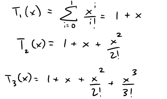
The graphs of the exponential function and these three Taylor polynomials are drawn in the figure below.
As n increases, Tn(x) appears to approach ex in the below figure.
This suggests that ex is equal to the sum of its Taylor series.
https://www.desmos.com/calculator/vqtlbufbnn
Retrieved: 17 January 2020
Archive: https://archive.ph/wip/EA87o

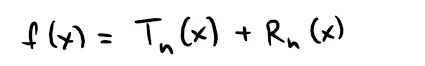
In general, f(x) is the sum of its Taylor series if:

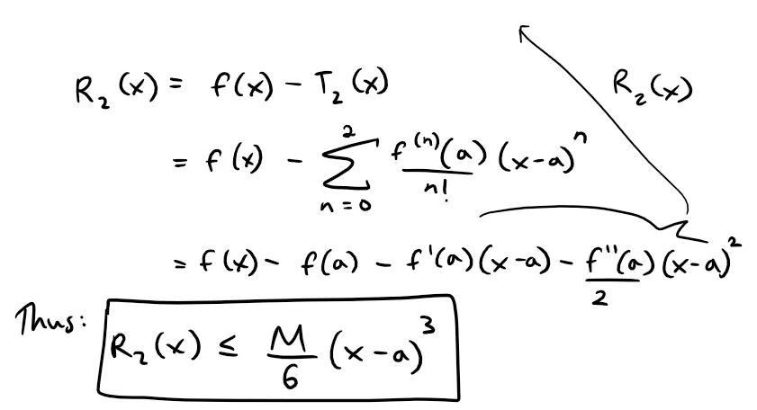
If we let:

then Rn(x) is called the remainder of the Taylor series.
If we can somehow show that:

then it follows that:
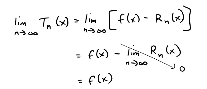
We have therefore proved the following theorem.
Theorem 2
If:
where Tn is the n-th degree Taylor polynomial of f at a and:
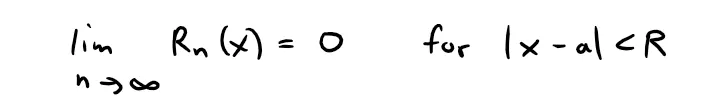
then f is equal to the sum of its Taylor series on the interval: |x - a| < R.
In trying to show that limn→∞ Rn(x) = 0 for a specific function f, we usually use the following fact:
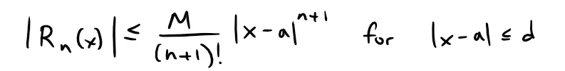
Taylor's Inequality
If:
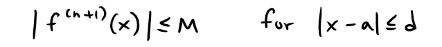
then the remainder Rn(x) of the Taylor series satisfies the inequality:
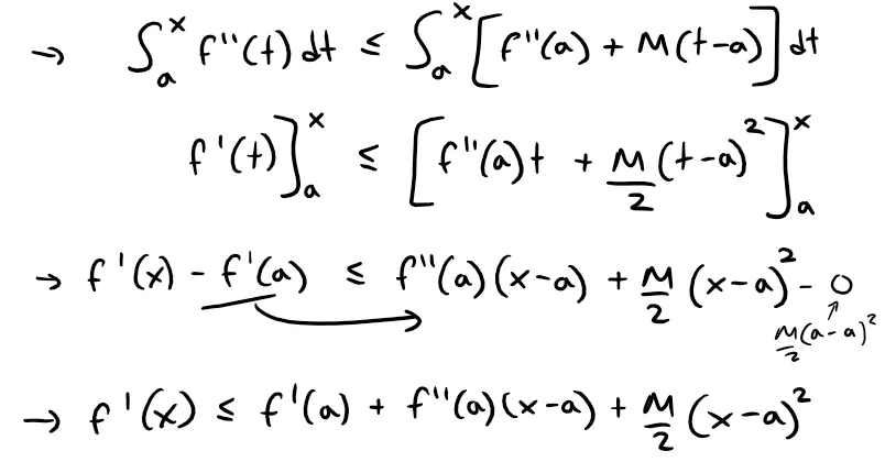
Proof of Taylor's Inequality for n = 1
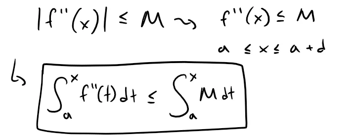
To see why this is true for n = 1, we assume that |f''(x)| ≤ M, which gives us the following two cases to consider:
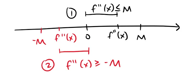
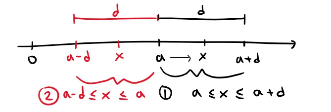
Likewise the interval |x - a| ≤ d also has the following two cases:
Thus, for f''(x) ≤ M and a ≤ x ≤ a + d, we have the integral inequality:
An antiderivative of f'' is f', so we can apply Part 2 of the Fundamental Theorem of Calculus referenced below.
Retrieved: 20 December 2019
Archive: https://archive.ph/wip/Bd7wE
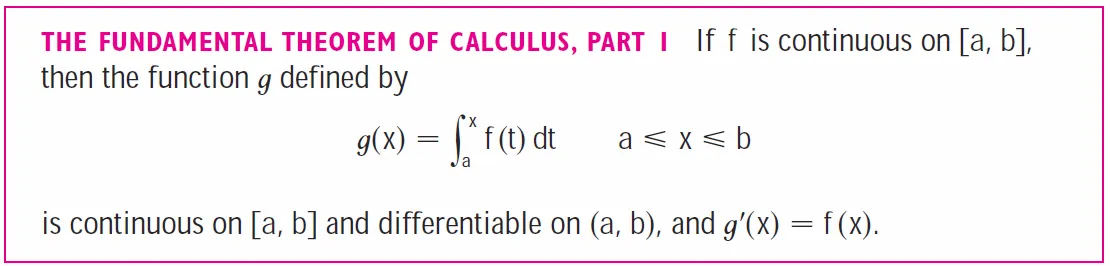
Retrieved: 20 December 2019
Archive: https://archive.ph/wip/AbsvX
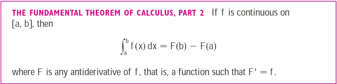
Thus we have:
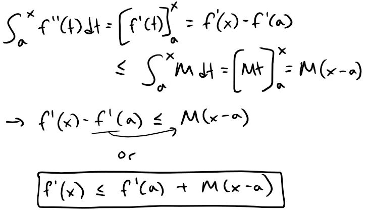
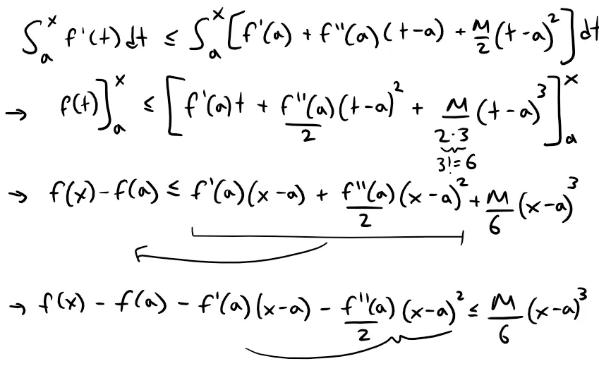
Repeating this process we get:

But:
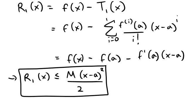
A similar argument, using f''(x) ≥ -M, shows that:

This is because we can just replace the f''(x) with -f''(x) in the earlier derivation.
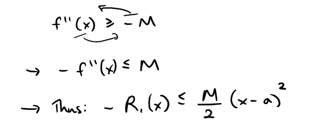
Thus:

Although we have assumed that x ≥ a, similar calculations show that this inequality is also true for x ≤ a.
This will just cause the integral to change signs and thus everything that follows will be the same but the signs changed; hence why this theorem is for the absolute value.

This proves Taylor's Inequality for the case where n = 1.
The result for any n is proved in a similar way by integrating n + 1 times.
See Exercise 2 at the end of this video for the case n = 2.
NOTE:
In later videos we will explore the use of Taylor's Inequality in approximating functions.
Our immediate use of it is in conjunction with Theorem 2.
In applying Theorem 2 and Taylor's Inequality it is often helpful to make use of the following fact:
Equation 1

This is true because we know from Example 1 that the series ∑ xn/n! converges for all x and so its n-th term approaches 0.
Note on Alternatives to Taylor's Inequality
As alternatives to Taylor's Inequality, we have the following formulas for the remainder term.
If f(n+1) is continuous on an interval I and x ϵ I, then:
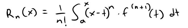
This is called the integral form of the remainder term.
Another formula, called Lagrange's form of the remainder term, states that there is a number z between x and a such that:
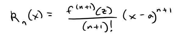
This version is an extension of the Mean Value theorem (which is the case n = 0).
I will go over the proofs of these "alternative" theorems for the remainder term in later videos.
Example 2
Prove that ex is equal to the sum of its Maclaurin series.
Solution:
If f(x) = ex, then as in Example 1, f(n+1)(x) = ex for all n.
If d is any positive number and |x - a| = |x - 0| = |x| ≤ d, then:
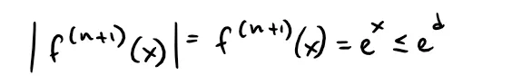
Since, ex is an increasing or exponential function that increases with increasing x.
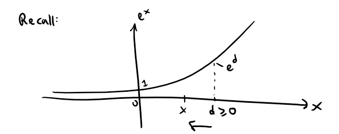
So Taylor's Inequality, with a = 0 and M = ed, says that:
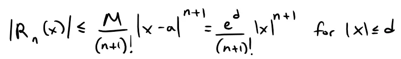
Notice that the same constant M = ed works for every value of n.
But, from Equation 1, we have:
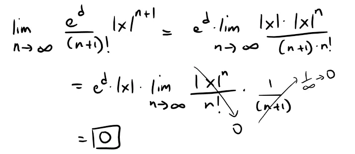
First recall from my earlier videos on the Squeeze Theorem in both conventional and sequences formulations.
Retrieved: 21 January 2020
Archive: https://archive.ph/wip/IyP35

@mes/infinite-sequences-limits-squeeze-theorem-fibonacci-sequence-and-golden-ratio-more
Retrieved: 21 January 2020
Archive: https://archive.ph/wip/kJR4R

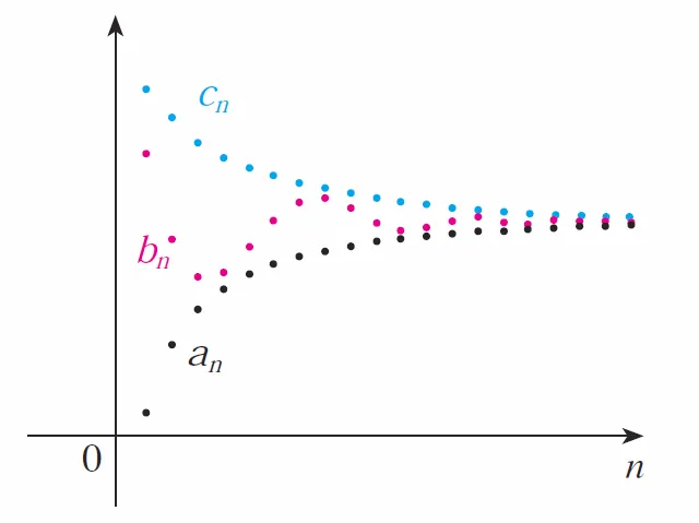
The sequence {bn} is squeezed between the sequences {an} and {cn}.
Thus, it follows from the Squeeze Theorem:

By Theorem 2, ex is equal to the sum of its Maclaurin series, that is:
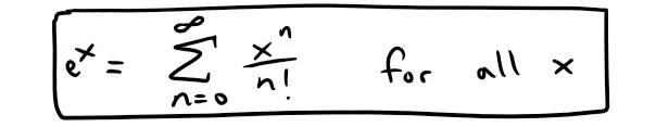
In particular, if we put x = 1 in the above series, we obtain the following expression for the number e as a sum of an infinite series:

Historical Note on Calculating the Number e
In 1748 Leonard Euler used the above to find the value of e correct to 23 digits.
In 2003 Shigeru Kondo, again using the series in above equation computed e to more than 50 billion decimal places.
The special techniques employed to speed up the computation are explained on the web page: http://numbers.computation.free.fr/Constants/constants.html
Example 3
Find the Taylor series for f(x) = ex at a = 2.
Solution:
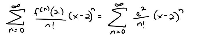
We have f(n)(2) = e2 and so, putting a = 2 in the definition of Taylor series, we get:
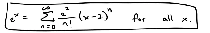
Again it can be verified, as in Example 1 since we are just replacing xn with (x - 2)n in the Ratio Test, that the radius of convergence is R = ∞.
Also as in Example 2 we can verify that limn→∞ Rn(x) = 0, which is again just replacing xn with (x - 2)n, so:
We have two power series expansions for ex, the Maclaurin series in Example 2 and the Taylor series in Example 3.
The first is better if we are interested in values of x near 0 and the second is better if x is near 2 (i.e. the terms of the series converge to 0 faster when x is near a).
Example 4
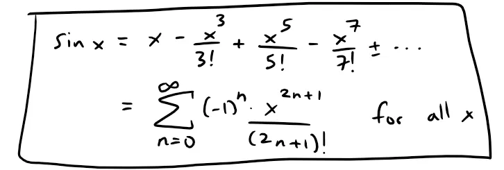
Find the Maclaurin series for sin x and prove that it represents sin x for all x.
Solution:
We arrange our computation in two columns as follows:
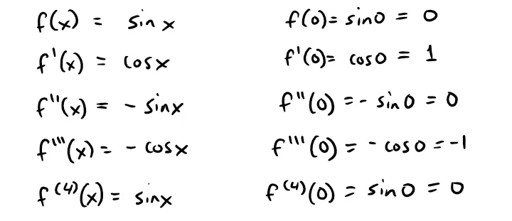
Since the derivatives repeat in a cycle of four, we can write the Maclaurin series as follows:

Since f(n+1) is ± sin x or ± cos x, we know that |f(n+1)(x)| ≤ 1 for all x.

So we can take M = 1 in Taylor's Inequality:
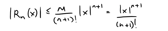
By Equation 1 the right side of this inequality approaches 0 as n → ∞, so |Rn(x)|→ 0 by the Squeeze Theorem.
It follows that Rn(x) → 0 as n → ∞, so sin x is equal to the sum of its Maclaurin series by Theorem 2.
We state the result of Example 4 for future reference.
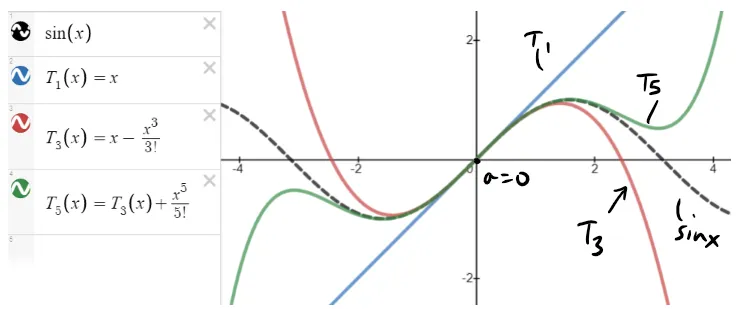
The following figure shows the graph of sin x together with its Taylor (or Maclaurin) polynomials:
Notice that, as n increases, Tn(x) becomes a better approximation to sin x.
https://www.desmos.com/calculator/wqhxcieee4
Retrieved: 22 January 2020
Archive: https://archive.ph/5CdBa

Example 5: cos x
Find the Maclaurin series for cos x.
Solution:
We could proceed directly as in Example 4 but it's easier to differentiate the Maclaurin series for sin x we just derived from Example 4:
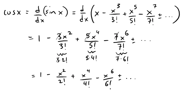
Since the Maclaurin series for sin x converges for all x, from my earlier referenced Theorem 1 from my earlier video tells us that the differentiated series for cos x also converges for all x; i.e. the radius of convergence is the same during term by term differentiation (or integration).
@mes/infinite-sequences-and-series-representations-of-functions-as-power-series
Thus:

Historical Note on Maclaurin Series
The Maclaurin series for ex, sin x, and cos x that we found in Examples 2, 4, and 5 were discovered, using different methods, by Newton.
These equations are remarkable because they say we know everything about each of these functions if we know all its derivatives at the single number 0.
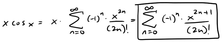
Example 6
Find the Maclaurin series for the function f(x) = x cos x.
Solution:
Instead of computing derivatives and substituting the f(n)(0) terms into the Maclaurin series equation, it's easier to multiply the series for cos x (which we just solved for in Example 5) by x:
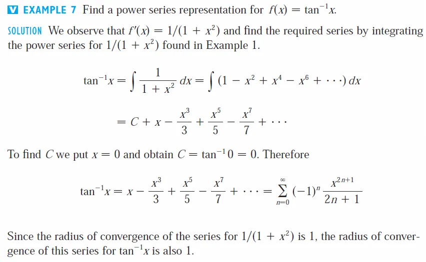
Example 7
Represent f(x) = sin x as the sum of its Taylor series centered at π/3.
Solution:
First, recall some exact trigonometric ratios:
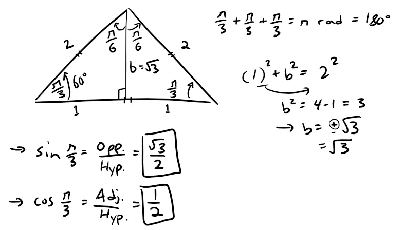
Arranging our work in columns, we have:
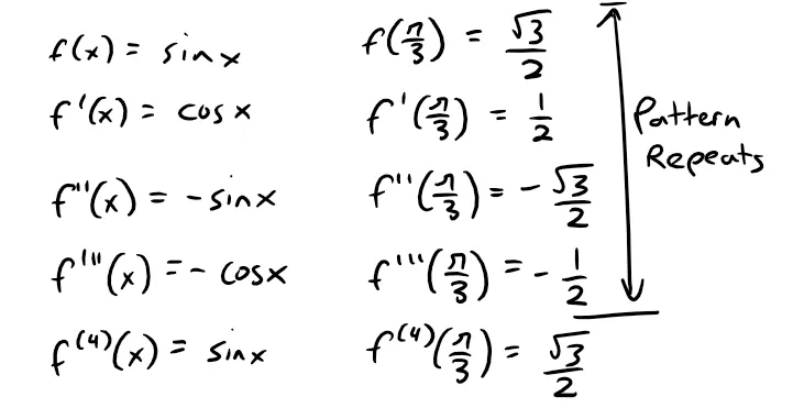
and this pattern repeats indefinitely.
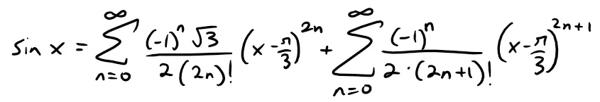
Therefore the Taylor series at π/3 is:

The proof that this series represents sin x for all x is very similar to that in Example 4.
Just replace x by x - π/3 in the Taylor Inequality.
We can write the series in sigma notation if we separate the terms that contain 31/2:
Note on Power Series
The power series that we obtained by indirect methods in Examples 5 and 6, and in my earlier video on representing functions as power series, are indeed the Taylor or Maclaurin series of the given functions because Theorem 1 asserts that, no matter how a power series representation f(x) = ∑ cn(x - a)n is obtained, it is always true that cn = f(n)(a)/n!.
In other words, the coefficients are uniquely determined.
Comparing Taylor and Maclaurin Series
We have obtained two different series representations for sin x, the Maclaurin series in Example 4 and the Taylor series in Example 7.
It is best to use the Maclaurin series for values of x near 0 and the Taylor series for x near π/3.
Notice that the third polynomial T3 in the figure below is a good approximation to sin x near π/3 but not as good as near 0.
https://www.desmos.com/calculator/vtebjpkndk
Retrieved: 24 January 2020
Archive: https://archive.ph/wip/r0nsM

Compare this with the third Maclaurin Polynomial T3 in the early Maclaurin series, where the opposite is true.
https://www.desmos.com/calculator/wqhxcieee4
Example 8: (1 + x)k
Find the Maclaurin series for f(x) = (1 + x)k, where k is any real number.
Solution:
Arranging our work in columns, we have:
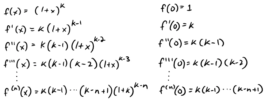
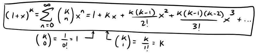
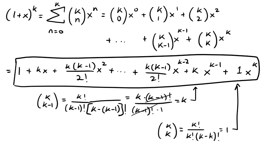
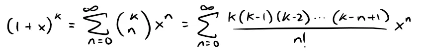
Therefore the Maclaurin series of f(x) = (1 + x)k is:
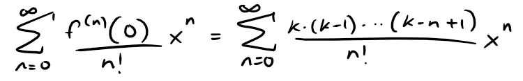
This series is called the binomial series.
If its n-th term is an, then applying the Ratio Test we get:
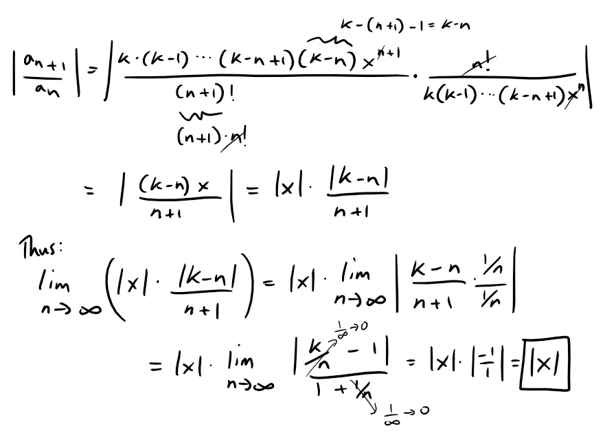
Thus, by the Ratio Test, the binomial series converges if |x| < 1 and diverges if |x| > 1.
The traditional notation for the coefficients in the binomial series is:
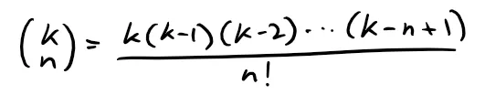
And these numbers are called the binomial coefficients.
Recall from my earlier video in which I went over a factorial expression for the binomial coefficients.
@mes/infinite-sequences-and-series-representations-of-functions-as-power-series
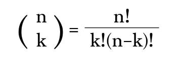
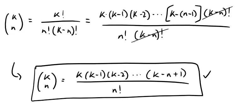
Where: n and k are both positive integers.
To get this factorial expression into our traditional notation we just need to switch the variables and do some factorial manipulations.
The following theorem states that (1 + x)k is equal to the sum of its Maclaurin series.
It is possible to prove this by showing that the remainder term Rn(x) approaches 0, but that turns out to be quite difficult.
The proof outlined in Exercise 3 at the end of this video is much easier.
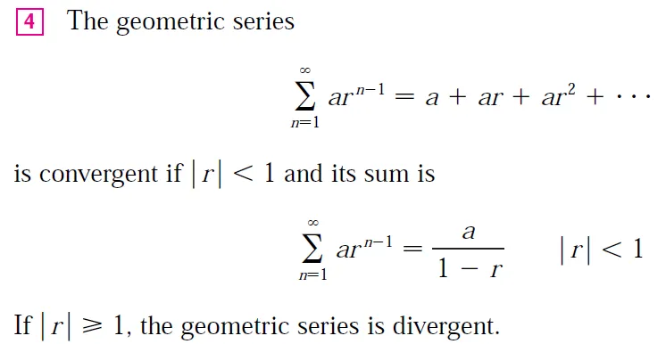
The Binomial Series
If k is any real number and |x| < 1, then:
Although the binomial series always converges when |x| < 1, the question of whether or not it converges at the endpoints ±1, (since the Ratio Test is inconclusive when the limit is equal to 1; in our case when |x| = 1) depends on the value of k.
It turns out that the series converges at 1 if -1 < k ≤ 0 and at both endpoints if k ≥ 0; I will look to prove this in another video as the proof is beyond what I have covered thus far.
Notice that if k is a positive integer and n > k, then the expression for (kn) contains a factor (k - k), so (kn) = 0 for n > k.
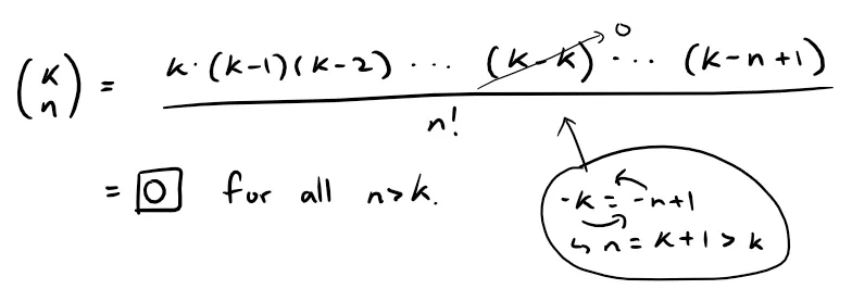
This means that the series terminates (i.e. remaining infinite terms are 0) and reduces to the ordinary Binomial Theorem when k is a positive integer, and the last non-zero term is at n = k.
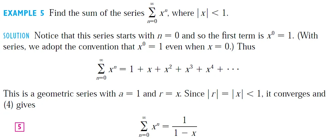
Example 9
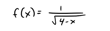
Find the Maclaurin series for the following function and its radius of convergence.
Solution:
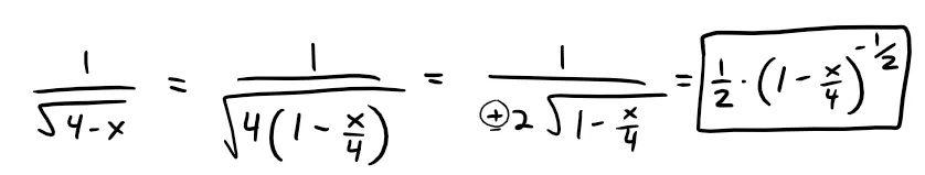
We write f(x) in a form where we can use the binomial series:
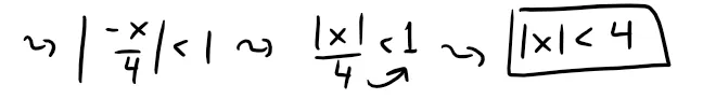
Using the binomial series with k = -1/2 and with x replaced by -x/4, we have:
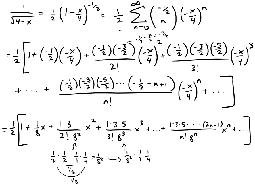
We know from the Binomial series (and derived from the Ratio Test) that this series converges when |-x/4| < 1, that is, |x| < 4, so the radius of convergence is R = 4.
We collect in the following table, for future reference, some important Maclaurin series that we have derived in this video and in my earlier videos.
Table 1: Important Maclaurin Series and Their Radii of Convergence
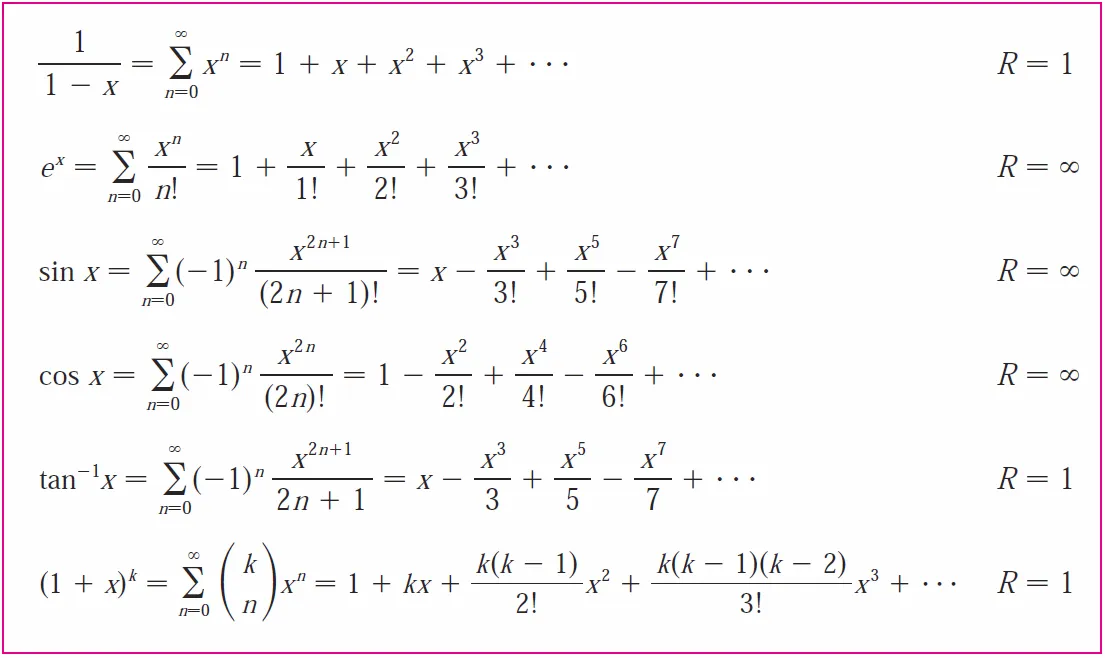
Note that the series for 1/(1 - x) and tan-1(x) were derived from my earlier videos referenced below.
@mes/infinite-series-definition-examples-geometric-series-harmonics-series-telescoping-sum-more
Retrieved: 27 July 2019
Archive: http://archive.fo/FGAyJ
@mes/infinite-sequences-and-series-representations-of-functions-as-power-series
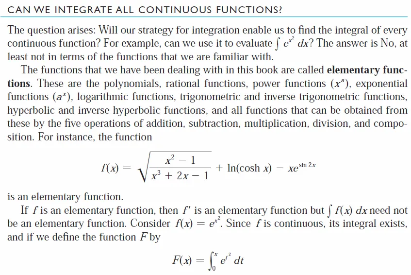
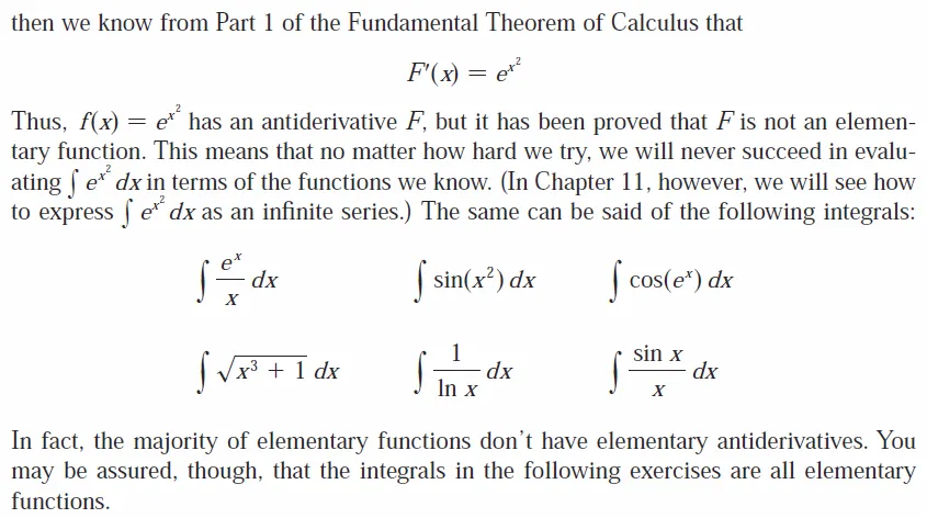
Integrating Functions that Don't Have Elementary Antiderivatives
One reason that Taylor series are important is that they enable us to integrate functions that we couldn't previously handle.
In fact, in the introduction to this chapter (in my first video on Infinite Sequences and Series) we mentioned that Newton often integrated functions by first expressing them as power series and integrating the series term by term.
The function:
can't be integrated by techniques discussed so far because its antiderivative is not an elementary function; as discussed in my earlier video which, interestingly enough, references this very same video you are watching! #VideoCeption
@mes/can-we-integrate-all-continuous-functions.
Retrieved: 27 January 2020
Archive: https://archive.ph/wip/lpu9G
In the following example we use Newton's idea to integrate this function.
Example 10
(a) Evaluate the following integral as an infinite series.

(b) Evaluate the following definite integral correct to within an error of 0.001.

Solution:
First we find the Maclaurin series for f(x) = e-x2.
Although it's possible to use the direct method, let's find it simply by replacing x with -x2 in the series for ex given in Table 1 and derived earlier in Example 2.
Thus, for all values of x,

Now we integrate term by term:
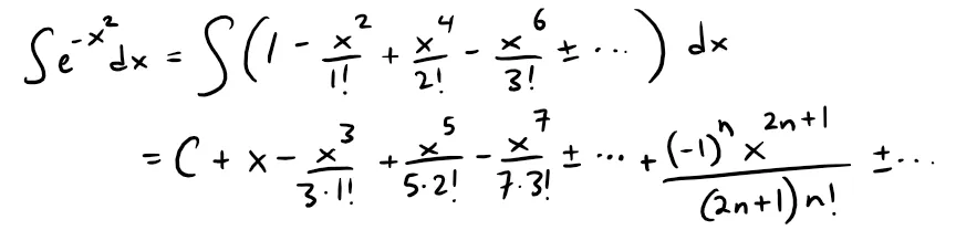
This series converges for all x because the original series for e-x2 converges for all x.
(b) The Fundamental Theorem of Calculus gives:
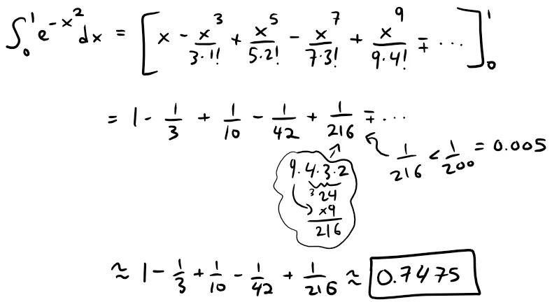
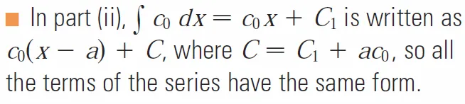
Note that we took C = 0 in the antiderivative from part (a).
Calculations Check:
- 1 - 1/3 + 1/10 - 1/42 + 1/216 = 0.7475
- 1/216 = 0.0046
- 1/200 = 0.005
To determine the accuracy of this estimation, we can use the Alternating Series Estimation Theorem referenced from my earlier below.
@mes/infinite-sequences-and-series-alternating-tests
Retrieved: 26 August 2019
Archive: http://archive.fo/9neM8
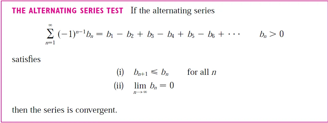
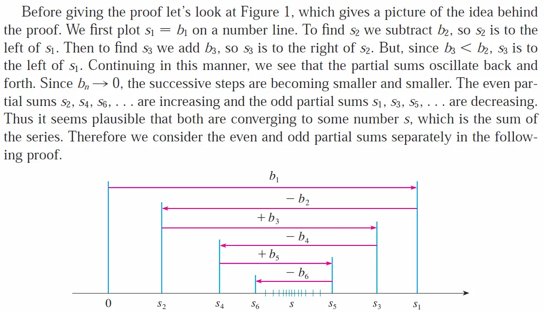
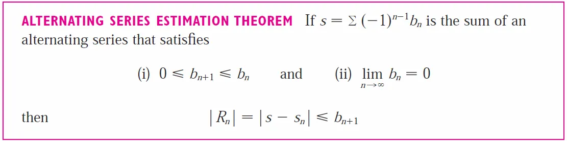

Thus the error, or Remainder, involved in this approximation is:
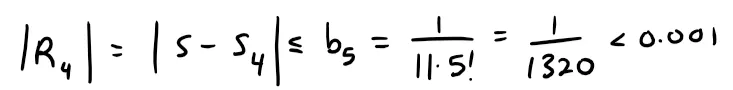
Calculations Check:
- 11*5! = 1,320
- 1/(11*5!) = 0.0008
- 1/1320 = 0.0008
- 1/1000 = 0.001
Another use of Taylor series is illustrated in the next example.
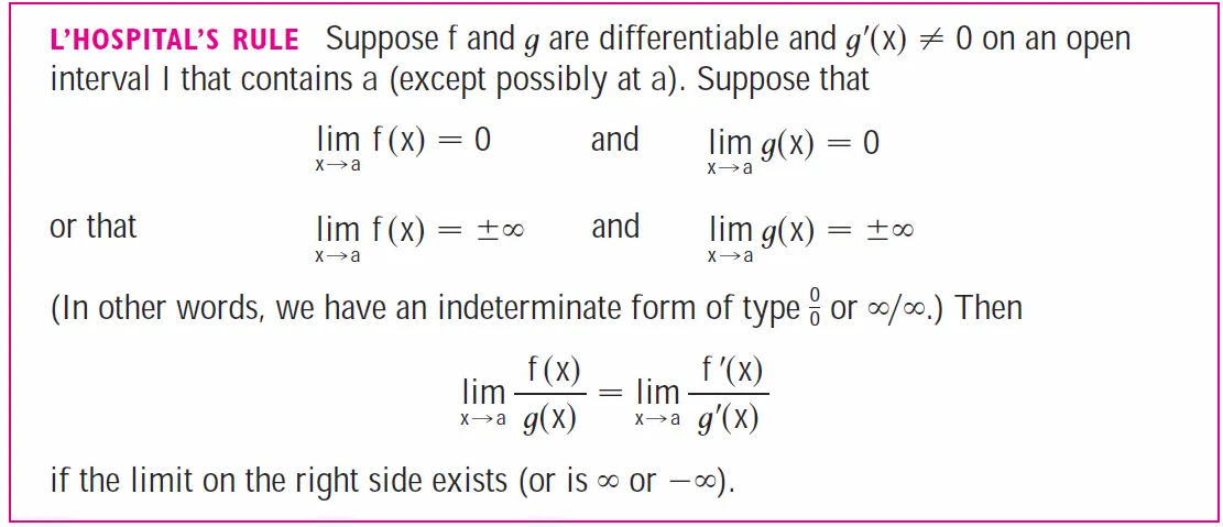
The limit could be found with L'Hospital's Rule, since it is an indeterminate limit of the form 0/0, but instead we use a series.
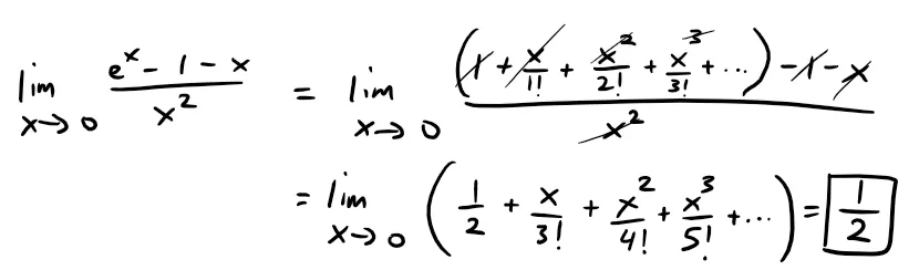
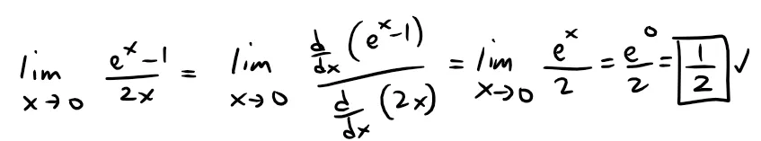
Example 11: Evaluating Limits
Evaluate the following limit:
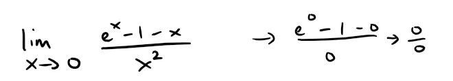
Solution:
Using the Maclaurin series for ex, we have:
Note that some computer algebra systems compute limits in this way.
Note also that we can take the limit of power series because they are continuous functions (since they are differentiable) as per my earlier video referenced below.
Retrieved: 22 December 2019
Archive: https://archive.ph/wip/w483w

As a double check we can find the limit by using L'Hospital's rule, referenced below.

Retrieved: 23 December 2019
Archive: https://archive.ph/wip/SKgVf
Thus we have:
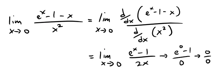
Applying L'Hospital's Rule again:
Multiplication and Division of Power Series
If power series are added or subtracted, they behave like polynomials, as shown in my earlier video referenced below.
@mes/infinite-series-definition-examples-geometric-series-harmonics-series-telescoping-sum-more
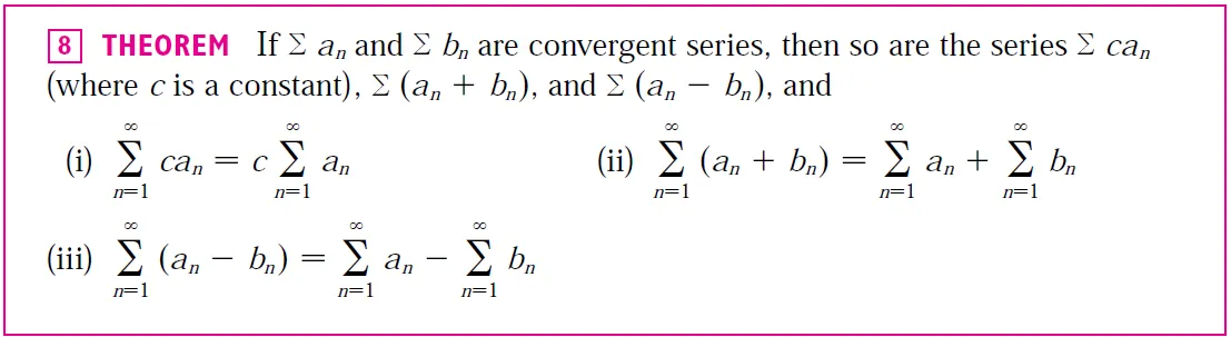
In fact, as the following example illustrates, they can also be multiplied and divided like polynomials.
We find only the first few terms because the calculations for later terms become tedious and the initial terms are the most important ones.
Example 12
Find the first three nonzero terms in the Maclaurin series for:
(a) ex sin x
(b) tan x.
Solution:
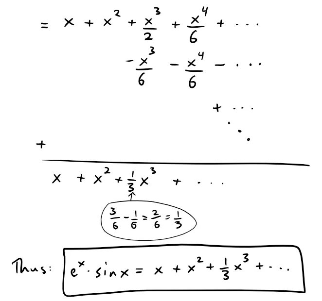
(a) Using the Maclaurin series for ex and sin x in Table 1, we have:
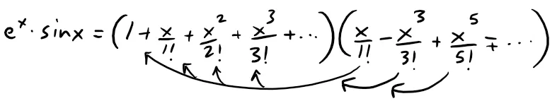
We multiply these expressions, collecting like terms just as for polynomials:
(b) Using the Maclaurin series in Table 1, we have:
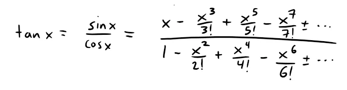
We use a procedure like long division:

Although we have not attempted to justify the formal manipulations used in Example 12, they are legitimate.
There is a theorem (which I will cover in a later video) which states if both f(x) = ∑ cnxn and g(x) = ∑ bn xn converge for |x| < R and the series are multiplied as if they were polynomials, then the resulting series also converges for |x| < R and represents f(x)g(x).
For division we require b0 ≠ 0; the resulting series converges for sufficiently small |x|.
Exercises
Exercise 1: A Function Not Equal to its Maclaurin Series
(a) Show that the function defined by:
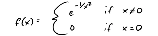
is not equal to its Maclaurin series.
(b) Graph the function in part (a) and comment on its behavior near the origin.
Solution:
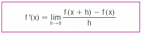
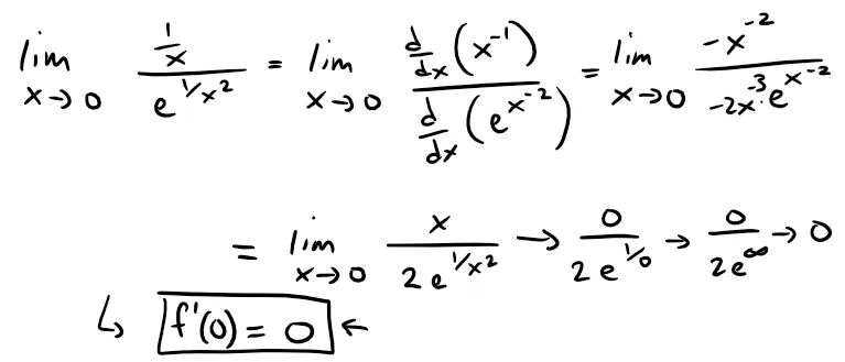
(a) Since the Maclaurin series is centered about 0, and the function f(x) consists of two distinct functions at x = 0 and x ≠ 0, to find the derivative f'(0) we first recall that the derivative is defined as a limit where, in this case, x → 0.
The definition of a derivative as a function is referenced below from my earlier video.

Retrieved: 22 December 2019
Archive: https://archive.ph/jVuBK
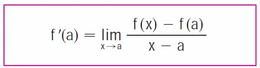
Thus with a = 0, we have:

Since this is indeterminate, we can apply L'Hospital's Rule:
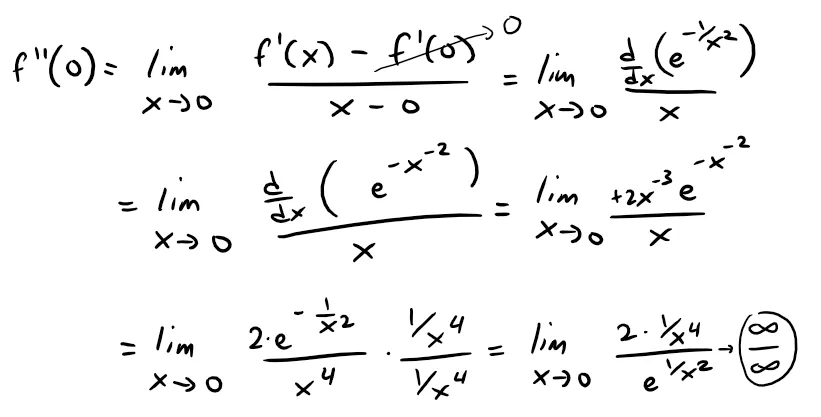
Similarly we can use the definition of the derivative and l'Hospital's Rule to show that f''(0) = 0, f(3)(0) = 0, … , f(n)(0) = 0.
For reference here is the derivation for f''(0) = 0.
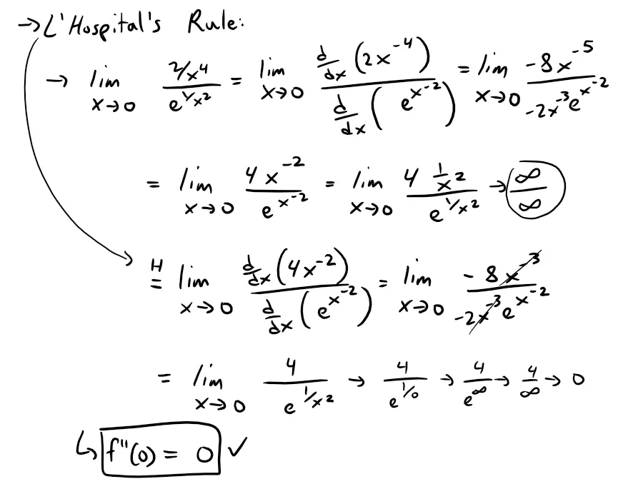
Thus the Maclaurin series for f consists entirely of zero terms.
But since f(x) ≠ 0 except for x = 0, we see that f cannot equal its Maclaurin series expect at x = 0.
(b) The graph of the function is shown below.
https://www.desmos.com/calculator/73ko0v3cxr
Retrieved: 4 February 2020
Archive: https://archive.ph/9gzi8
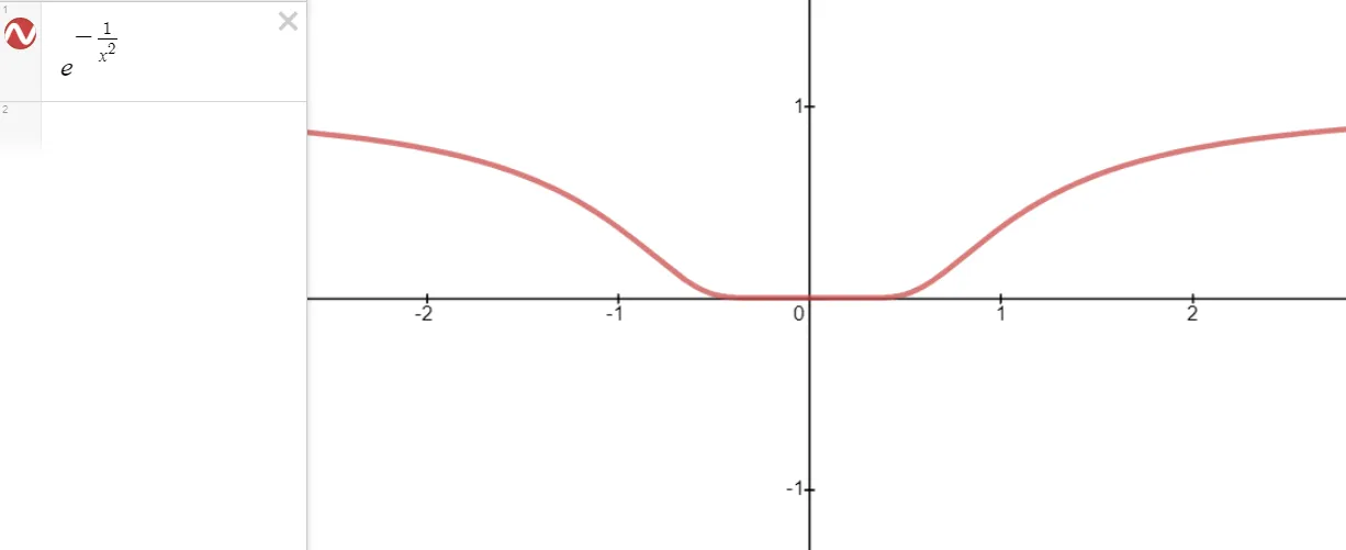
Zooming in even closer we get the following graph.
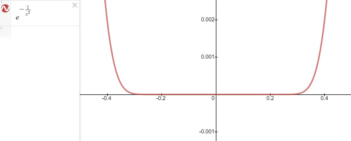
From the graph, it seems that the function is extremely flat at the origin.
In fact, it could be said to be "infinitely flat" at x = 0, since all of its derivatives are 0 there.
Exercise 2
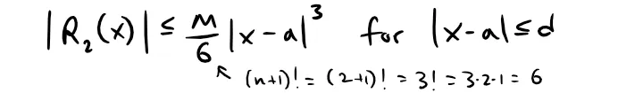
Prove Taylor's Inequality for n = 2, that is, prove that if:

then:
Solution:
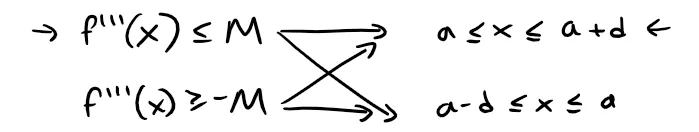
Assume that |f'''(x)| ≤ M for |x - a| ≤ d, and in particular we have the following cases, as in the earlier derivation for n = 1:
Thus, for f'''(x) ≤ M and a ≤ x ≤ a + d, we have the integral inequality:
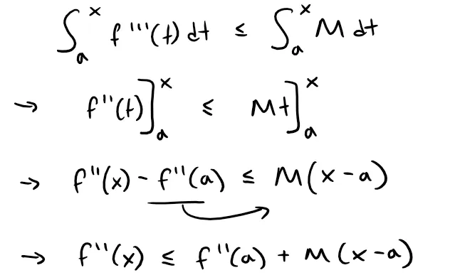
Repeating the process we get:
Repeating the process one more time we get:
But:
A similar argument, using f'''(x) ≥ - M shows that:
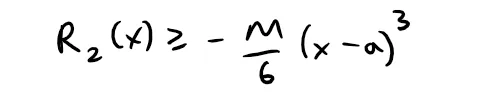
Thus:

Although we derived for the case x ≥ a, similar calculations show that this inequality is also true if x ≤ a.
Exercise 3
Use the following steps to prove the Binomial Series, that is to prove (1 + x)k is equal to its Maclaurin series, with |x| < 1:
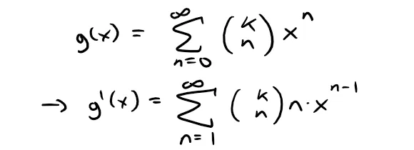
(a) Let:
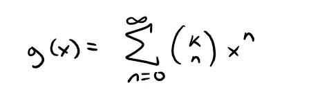
Differentiate this series to show that:

(b) Let h(x) = (1 + x)-k g(x) and show that h'(x) = 0.
(c) Deduce that g(x) = (1 + x)k.
Solution:
(a) Differentiating the power series we get:
Now to get it in the form asked of us, we can multiply both sides by (1 + x).

To get both sides with a xn power, we can replace n with n + 1 in the first series (and start with n = 0 in the second series which merely means a 0 term).
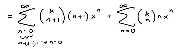
Expanding the binomial expression we get:
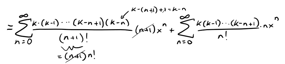
Factoring out the like terms and combining into one series we get:
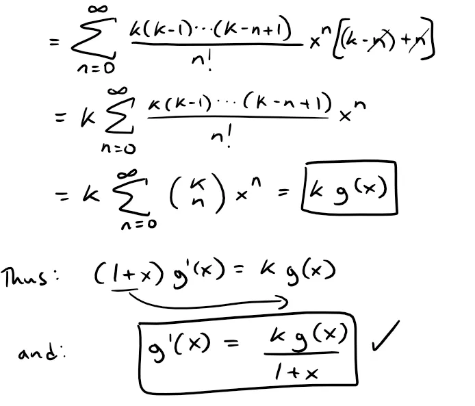
Recall from Example 8 that the binomial series converges for |x| < 1 thus the derivative of a binomial series, which is a just a power series, also converges for |x| < 1, that is for - 1 < x < 1.
Thus:
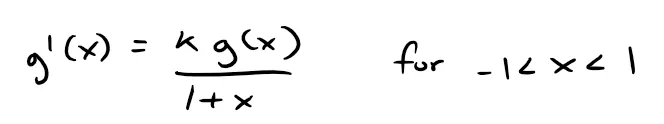
Note that at the endpoints x = ± 1, convergence depends on the k value.
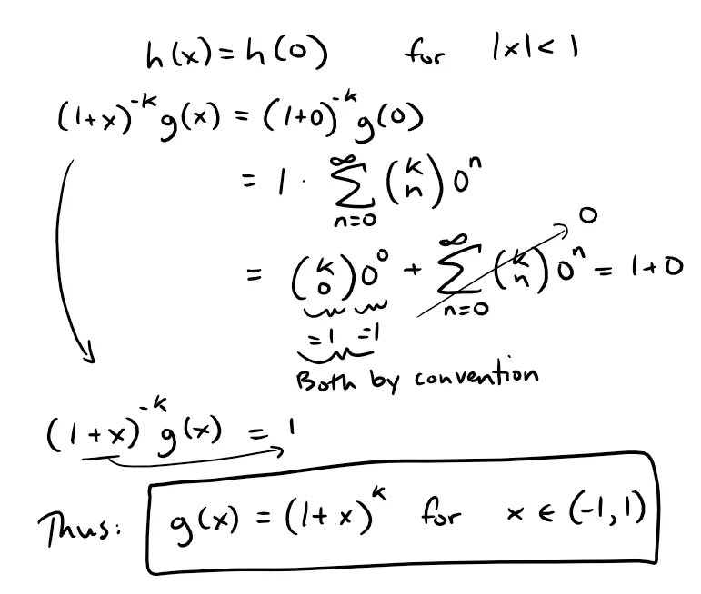
(b) Taking the derivative of h(x) we get:
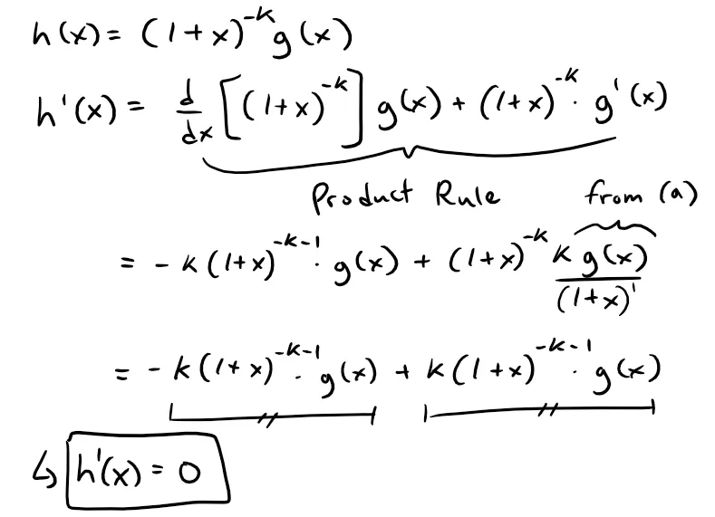
(c) From part (b) we see that h(x) must be constant for x ϵ (-1 , 1), or |x| < 1, since the rate of change, or derivative, is equal to 0, that is: h'(x) = 0.
This means that we can choose any value of |x| < 1 and h(x) will be the same, thus simply choosing x = 0, we get: