
Introduction
PYroMat is an open source program that provides us with thermodynamic properties in Python. PYroMat; used to obtain the thermodynamic properties of materials from the command line or command line files. It says will always be free and open. Most of PYroMat's 400+ species are ideal gases. PYroMat says there are alternative programs that do similar work, but all of them are either for profit, have limited capabilities, are devoted to much narrower data sets, or are built to perform a specific job.
The refrigerants and some important substances like nitrogen, oxygen, and carbon dioxide are the basic functions of the PYroMat. Cycles is the most important in the PYromat like Brayton and Rankine cycles. These cycles are important air circles and benefit from Pyromat's refrigeration function.
Today we will concentrate on the Bryton cycle. The Bryton cycle is basically a refrigeration machine. The fluid flowing in this system is air. The air is a gas mixture and we consider it an ideal gas in this system. We will create P-v and T-s diagrams with the help of PYroMat.
What Will I Learn?
How to build Bryton cycle P-v and T-s diagrams with PYroMat?
- You will learn how to use PYroMat function ?
- You will learn how to build Bryton formulas ?
- You will learn how to build Bryton P-V diagram ?
- You will learn how to build Bryton T-S diagram ?
Requirements
PYroMat you can access it here
Python 3.6
Python Shell (Comes with Python 3.6) or another command tool
Matplotlib
Difficulty
- Basic
Tutorial Contents
Features of PYroMat
PYroMat offers thermodynamic properties for about 400 substances to us. Includes the following features:
- ‘cp’ Isobaric specific heat
- ‘cv’ Isochoric specific heat
- ‘d’ Density
- ‘e’ Internal energy
- ‘gam’ Specific heat ratio
- ‘h’ Enthalpy
- ‘mw’ Molecular weight
- ‘R’ Ideal gas constant
- ‘s’ Entropy
We will import PYroMat first for use it. For that, we will use the following command:
import pyromat as pyro
We will import numpy to use it. For that, we will use the following command:
import numpy as np
Now we will import matplotlib to do graphics. For that, we will use the following command:
import matplotlib.pyplot as plt
The Bryton Cycle is an air cycle. Here, air is used as a refrigerant in the cycle. The Brayton refrigeration cycle consists of 4 state changes:
(1-2): Adiabatic compression in compressor,
(2-3): Refrigeration of air at constant pressure,
(3-4): Reversible adiabatic expansion in turbin,
(4-1): Heat conduction from air to refrigate air at constant pressure.
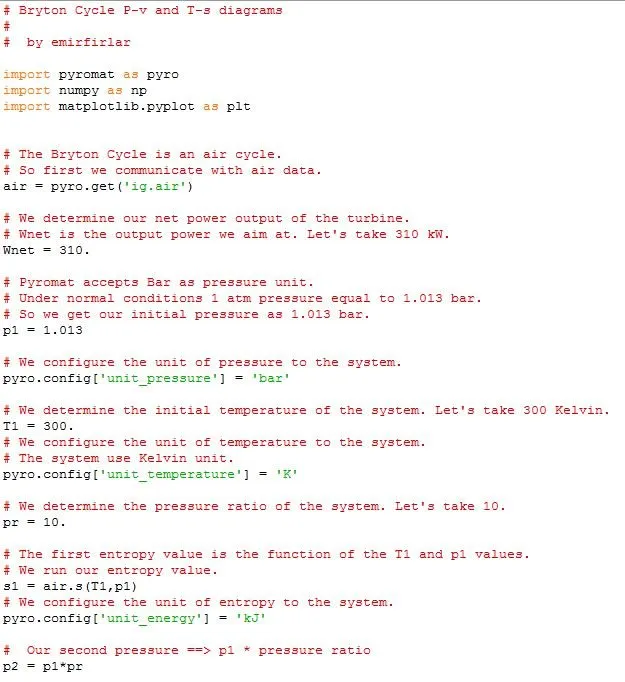
So first, we communicate with air data. For that, we will use the following command:
air = pyro.get('ig.air')
At first, We determine our net power output of the turbine. Wnet is the output power we aim at. Let's take 310 kW. For that, we will use the following command:
Wnet = 310.
PYroMat accepts Bar as pressure unit. Under normal conditions 1 atm pressure equal to 1.013 bar. So we get our initial pressure as 1.013 bar. For that, we will use the following command:
p1 = 1.013
We will configure the unit of pressure to the system. For that, we will use the following command:
pyro.config['unit_pressure'] = 'bar'
We determine the initial temperature of the system. Let's take 300 Kelvin. For that, we will use the following command:
T1 = 300.
We configure the unit of temperature to the system. The system use Kelvin unit. For that, we will use the following command:
pyro.config['unit_temperature'] = 'K'
We determine the pressure ratio of the system. Let's take 10. For that, we will use the following command:
pr = 10.
The first entropy value is the function of the T1 and p1 values. We run our entropy value. For that, we will use the following command:
s1 = air.s(T1,p1)
We configure the unit of entropy to the system. For that, we will use the following command:
pyro.config['unit_energy'] = 'kJ'
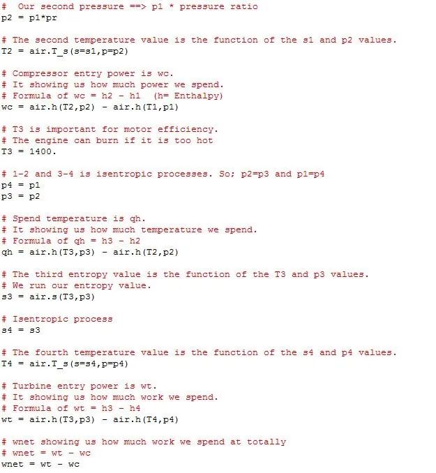
Our second pressure ==> p1 * pressure ratio. For that, we will use the following command:
p2 = p1*pr
The second temperature value is the function of the s1 and p2 values. For that, we will use the following command:
T2 = air.T_s(s=s1,p=p2)
Compressor entry power is wc. It showing us how much power we spend. Formula of wc = h2 - h1 (h= Enthalpy) For that, we will use the following command:
wc = air.h(T2,p2) - air.h(T1,p1)
T3 is important for motor efficiency. The engine can burn if it is too hot. For that, we will use the following command:
T3 = 1400.
(1-2) and (3-4) are isentropic processes. So; will be p2=p3 and p1=p4. For that, we will use the following command:
p4 = p1
p3 = p2
Spend temperature is qh. It showing us how much temperature we spend. Formula of qh = h3 - h2 . For that, we will use the following command:
qh = air.h(T3,p3) - air.h(T2,p2)
The third entropy value is the function of the T3 and p3 values. We run our entropy value. For that, we will use the following command:
s3 = air.s(T3,p3)
s4 = s3 must be. Because this is isentropic process. For that, we will use the following command:
s4 = s3
The fourth temperature value is the function of the s4 and p4 values. For that, we will use the following command:
T4 = air.T_s(s=s4,p=p4)
Turbine entry power is wt. It showing us how much work we spend. Formula of wt = h3 - h4. For that, we will use the following command:
wt = air.h(T3,p3) - air.h(T4,p4)
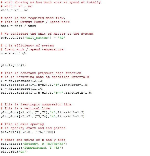
wnet showing us how much work we spend at totally. For that, we will use the following command:
wnet = wt – wc
mdot is the required mass flow. This is Output Power / Spend Work. For that, we will use the following command:
mdot = Wnet / wnet
We configure the unit of matter to the system. For that, we will use the following command:
pyro.config['unit_matter'] = 'kg'
n is efficiency of system. Efficiency is spend work / spend temperature. For that, we will use the following command:
n = wnet / qh
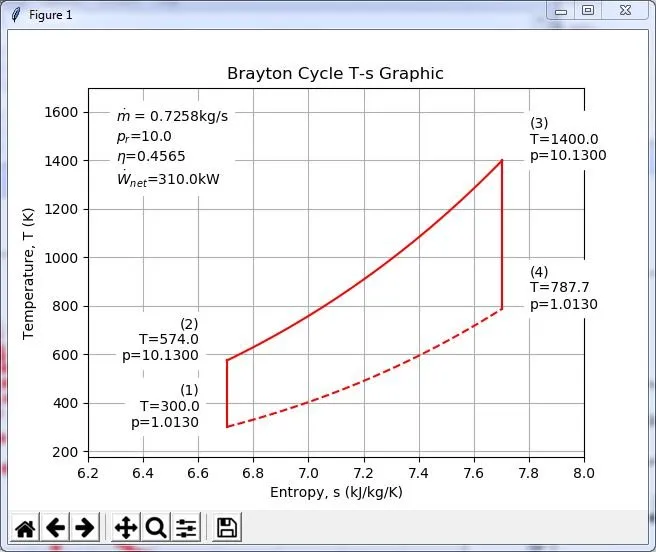
So far we have defined the formulas of the bryton cycle. We looked at how to import them. Now we will first build the T-s diagram. T-S diagram has a specific shape. In this diagram, we will build two separate sections. These are constant pressure heat function and isentropic compresion line.
We will build constant pressure heat function. It consists of parts a(2-3) and (1-4). It is returning data at specified intervals. Numpy gives us this feature. For that, we will use the following command:
T = np.linspace(T2,T3)
plt.plot(air.s(T=T,p=p2),T,'r',linewidth=1.5)
T = np.linspace(T1,T4)
plt.plot(air.s(T=T,p=p1),T,'r--',linewidth=1.5)
Now we will build isentropic compresion line. This is a vertical line. It consists of coordinates (s1,T1), (s1,T2) and (s3,T3), (s3,T4). For that, we will use the following command:
plt.plot([s1,s1],[T1,T2],'r',linewidth=1.5)
plt.plot([s3,s3],[T3,T4],'r',linewidth=1.5)
We will finally define the axis bounds for this diagram. It specify start and end points. For that, we will use the following command:
plt.axis([6.2,8 , 175,1700])
We will give names to the x and y axes. For that, we will use the following command:
plt.xlabel('Entropy, s (kJ/kg/K)')
plt.ylabel('Temperature, T (K)')
plt.grid('on')
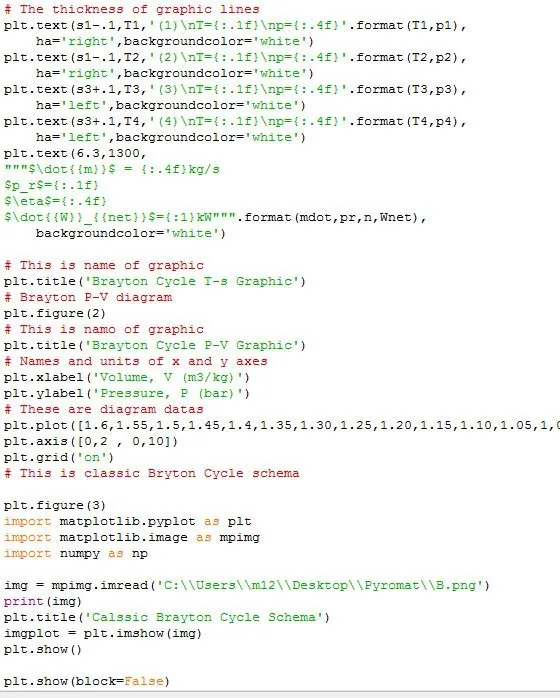
We will adjust thickness of graphic lines and text. I preferred 1f and 4f. You can choose 3f or 6f if you want. I used white background. You can change this with another color if you want. For that, we will use the following command:
plt.text(s1-.1,T1,'(1)\nT={:.1f}\np={:.4f}'.format(T1,p1),
    ha='right',backgroundcolor='white')
plt.text(s1-.1,T2,'(2)\nT={:.1f}\np={:.4f}'.format(T2,p2),
    ha='right',backgroundcolor='white')
plt.text(s3+.1,T3,'(3)\nT={:.1f}\np={:.4f}'.format(T3,p3),
    ha='left',backgroundcolor='white')
plt.text(s3+.1,T4,'(4)\nT={:.1f}\np={:.4f}'.format(T4,p4),
    ha='left',backgroundcolor='white')
plt.text(6.3,1300,
"""$\dot{{m}}$ = {:.4f}kg/s
$p_r$={:.1f}
$\eta$={:.4f}
$\dot{{W}}_{{net}}$={:1}kW""".format(mdot,pr,n,Wnet),
    backgroundcolor='white')
We will finish typing T-S diagram by typing of name. For that, we will use the following command:
plt.title('Brayton Cycle T-s Graphic')
We our output diagram will be as follows:
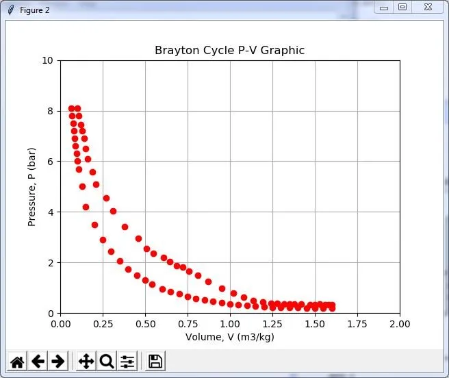
Now we can build the P-V diagram. We must first call our code for the second chart . Then we will upload the data. P-V diagram consists of point coordinates. We need to load the diagram data for this. For that, we will use the following command:
plt.figure(2)
plt.plot([x1,x2],[y1,y2])
Now, we will build the limits. For that, we will use the following command:
plt.axis([0,2 , 0,10])
plt.grid('on')
We will name axes and diagram. . For that, we will use the following command:
plt.title('Brayton Cycle P-V Graphic')
plt.xlabel('Volume, V (m3/kg)')
plt.ylabel('Pressure, P (bar)')
We our output diagram will be as follows:
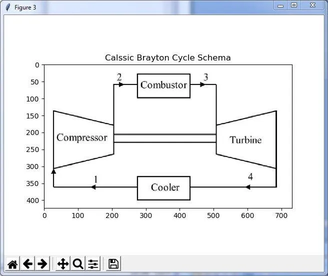
We successfully built our P-v diagram. We will load the classic Bryton cycle diagram to understand how the Brayton cycle works. I will import the picture I made earlier as png. Matplotlib gives us this feature. I use the this codes for this:
plt.figure(3)

import matplotlib.pyplot as plt
import matplotlib.image as mpimg
import numpy as np

img = mpimg.imread('C:\\Users\\m12\\Desktop\\Pyromat\\B.png')
print(img)
plt.title('Calssic Brayton Cycle Schema')
imgplot = plt.imshow(img)
plt.show()
We our output diagram will be as follows:
We will add the following command after you have written all the codes:
plt.show(block=False)
Thus we are finishing P-V, T-S and schema construction.
You can see the all of output in the system in detail below on gif:

Below you can see the all of codes in their entirety:
Today we used the open-source thermodynamic property program Pyromat. We benefitted pyromat's brayton cycle feature. We built P-v and T-S diagrams.
Thank you for following the lesson !
Source:
1,
2,
3,
Github repository
Posted on Utopian.io - Rewarding Open Source Contributors