
#1 – Make a Duplicate Copy of a Worksheet
This first one I use A LOT. Especially when I want to create a backup copy of a sheet or duplicate a sheet so I can make changes without screwing up the original.
The quickest way I’ve found to make a duplicate copy of a sheet is to:
1.Left-click and hold on the sheet you want to copy.
2.Press and hold the Ctrl key. A plus symbol will appear in the sheet mouse icon.
3.Drag the sheet to the right until the down arrow appears to the right of the sheet.
4.Release the left mouse button. Then release the Ctrl key.
It sounds like a lot, but once you get the hang of it you will wonder how you ever lived without this trick. It’s much faster than right-clicking the tab and going to the Move or Copy… menu.
You can also first select multiple sheets with the Shift key, then use the same method to copy multiple sheets at the same time.
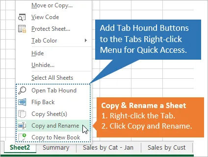
My Tab Hound add-in also has a feature that adds a command to the sheet tab’s right-click menu to make a duplicate copy of the sheet with one click.
Bonus tip: This Ctrl & Drag method also works to make duplicate copies of shapes or charts. Select a shape/chart and then hold Ctrl while moving it. Release the mouse button and a copy of the object will be placed on the sheet. Release the Ctrl key after releasing the mouse button.
#2 – Ctrl+Enter to Fill Multiple Cells
This keyboard shortcut can save time when entering the same formula in multiple cells.
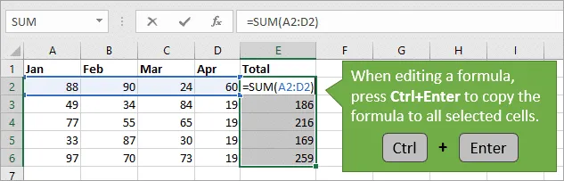
1.Select the cells that the formula will be inserted in.
2.Type or insert the formula or text in the active cell.
3.Hold the Ctrl key and press Enter.
The formula or text will be copied to all the selected cells.
Mac shortcut: Ctrl+Enter or Cmd+Enter
As you probably know, there are a TON of ways to copy or fill formulas. This technique works best when you already have the range selected that you want to insert or modify formulas in. This tends to happen when we are modifying formulas or fixing them for errors.
#3 – Ctrl+T to Create a Table
If you are using Excel Tables then you won’t need the Ctrl+Enter shortcut as often. That’s because Excel Tables automatically fill the formulas down a column for you.
It’s just one of the many great benefits of using Excel Tables. I’m a huge fan of them.
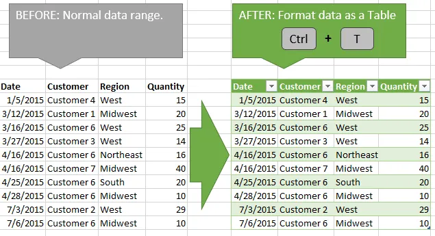
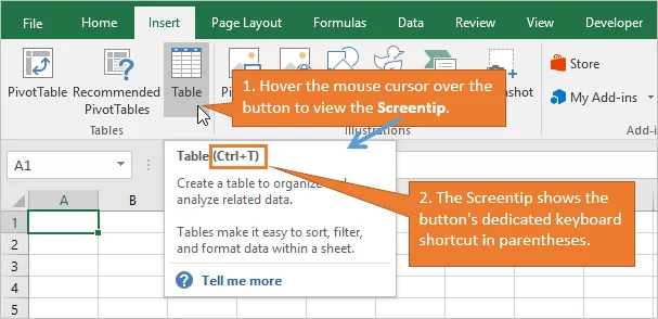
The keyboard shortcut to format your data as a Table is Ctrl+T. The shortcut is different in different language versions of Excel, so hover over the Table button on the Insert tab of the ribbon to see what the shortcut is for you.
#4 – Apply & Clear Table Formatting
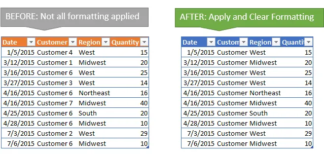
One nice feature of Excel Tables is the styling or formatting that is applied when you insert the Table. You can quickly make your data look very nice and organized. Every other row of the Table is shaded (banded) to give it a clean look that is easier to read.
If your range already has some formatting in the header row, then sometimes your Table can look a little ugly after creating it. The Table formatting does not get fully applied to the header row for some reason.
Fortunately, there is a quick fix:
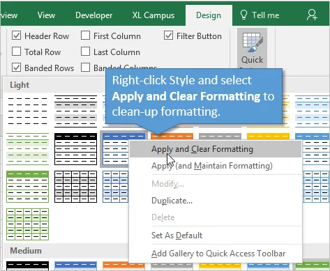
1.Select a cell inside the Table.
2.Go to the Design tab in the Ribbon.
3.Right-click one of the Table styles in the Styles Gallery.
4.Choose Apply & Clear Formatting.
5.This will clear all the existing formatting in the range and apply the Table style.
#5 – AutoFit Column Width
After entering a formula, inserting a Table, or pasting data, your column widths might need to be adjusted to fit the new contents.
The keyboard shortcut to auto fit the column widths is: Alt,h,o,i
Press and release each key in order.
Bonus tip: You can do this all in one step by going to the Home tab of the ribbon, clicking the Format as Table drop-down, and right-click>Apply & Clear Formatting on any style. This will create the Table for your range and clear the existing formatting all at the same time.
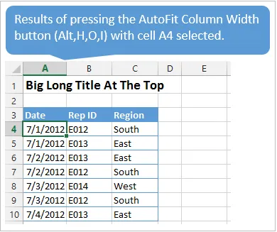
This will automatically expand the width of the column to fit the contents of the cells that are currently selected. This is important to note. If you want to resize the column to only fit a specific cell or group of cells, then select those cells first and press the keyboard shortcut.
Mac shortcut: Unfortunately the 2016 version for Mac does not have the Alt key shortcut combinations. I don’t believe there is a shortcut key for this. Please leave a comment below if you know it.
#6 – Select the Corners of a Range
Have you ever pasted some data over existing data, then wondered if the new data is long enough or wide enough to paste over the existing data?
If so, the Ctrl+. (period) keyboard shortcut will save you from scrolling all the way down the sheet.
Pressing Ctrl+. (hold the Ctrl key and press the period key) will select the next corner of the selected range. After pasting a range of data, press Ctrl+. to select the top-right cell of the selected range. Then press Ctrl+. again to select the bottom-right cell.
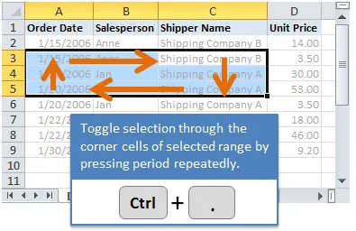
This will get you down to the bottom of the pasted range where you can quickly see if you pasted over the existing data.
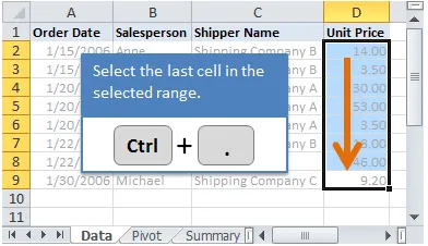
You can also use this shortcut to jump down to the bottom of a single column.
Mac shortcut: Ctrl+. (same as Windows)
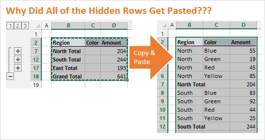
#7 – Select Visible Cells
When our data contains hidden rows or columns, or has filters applied, copy and paste can produce unexpected results. Sometimes we copy a range expecting to only copy the visible cells. Then when we paste, all of the hidden rows or columns are pasted too. Argh!
When this happens, we first need to select the visible cells. The keyboard shortcut to select visible cells is Alt+; (semicolon). Press this shortcut key after selecting the range, to only select the visible cells.
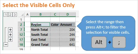
Mac shortcut: Cmd+Shift+Z
#8 – Go To a Range from a Formula
When editing formulas with range references on other sheets, it can sometimes be difficult to navigate to those sheets to find the range. Especially when your workbook has a lot of sheets.
One quick tip to navigate to a range on another sheet is to:
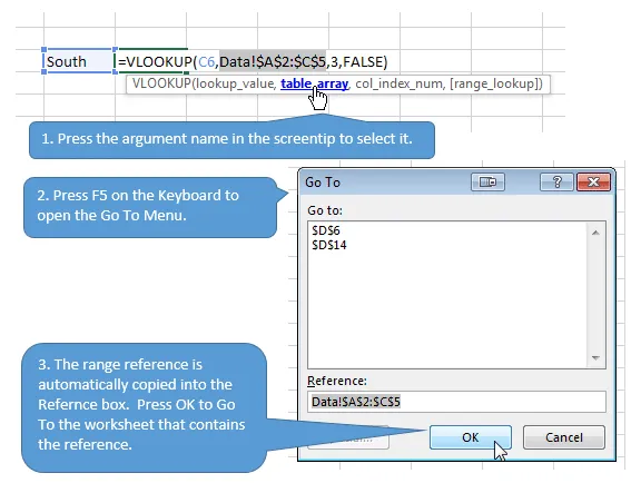
1.Select the sheet and range reference in the formula with the screentip hyperlink.
2.Press F5 or Ctrl+G on the keyboard to open the GoTo Window. The sheet and range reference will be placed in the Reference box.
3.Hit Enter or OK to go to that sheet and see the range selected.
Mac shortcut: F5 or Ctrl+G (same as Windows).
#9 – 3 Uses for Alt+Down Arrow
The Alt+Down Arrow keyboard shortcut opens drop-down menus. This works in Excel and most other applications as well (including web browsers).
To perform the shortcut you simply hold down the Alt key and press the down arrow key on the keyboard. Here’s what it can do in Excel
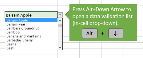
#1 – Open data validation lists (in-cell drop-down lists)
Select a cell that contains data validation and press Alt+Down Arrow to open the data validation list.
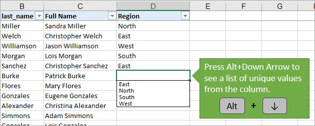
#2 – Create a drop-down list of items in a column
If the cell does NOT contain data validation, then we can press Alt+Down Arrow to create a drop-down list of all the unique items in that column. This is great for doing data entry because it allows you to select from a list of items in the column, and prevents typos.
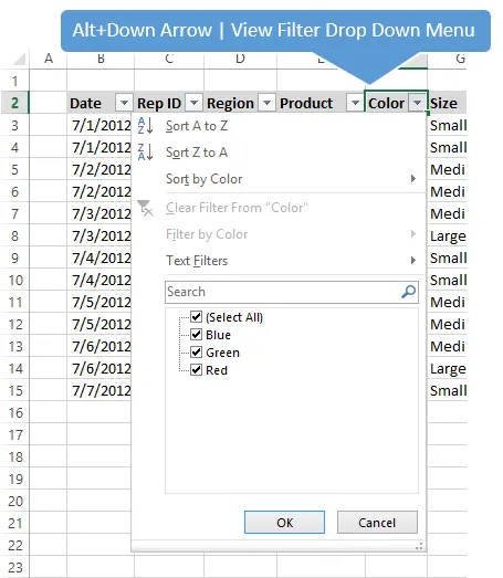
#3 – Open the Filter Drop-down Menu
Select a cell in the header row of a filtered range and press Alt+Down Arrow to open the filter drop-down menu.
Mac shortcut: Alt+Down Arrow works the same on the Mac for all 3 tips above.
#10 – Lock Drawing Mode to Create Multiple Shapes=
Have you ever wanted to draw a bunch of the same shape (lines, boxes, circles) on a sheet, and repeatedly had to go to the Insert >Shapes menu? If so, this little shortcut can save a bunch of time.
1.Go to the Insert tab and press the Shapes menu.
2.Right-click the shape you want to insert.
3.Select “Lock Drawing Mode”.
4.Draw the shape on the sheet
5.Then draw another shape. You can continue to draw as many of the same shape as you’d like
The drawing mode is locked and it will continue to let you draw multiple shapes. Hit the Escape key on the keyboard when you are done.
Mac shortcut: I don’t believe there is any way to lock drawing mode on the Mac version. Please leave a comment below if you know of one.
#11 – Lock the Format Painter
The Format Painter is one of those handy tools that allows us to quickly copy and paste the formatting of an object. This can be a cell, shape, chart, pivot table, etc.
It’s a very simple tool to use.
1.Select the object you want to copy the formatting from.
2.On the Home tab of the ribbon, press the Format Painter button.
3.Then select the object you want to paste the formatting to.
Now, what if you want to apply formatting to more than one object. In step 2 above, double-click the Format Painter button. This will lock the format painter and allow you to select multiple objects to apply formatting to.
When finished, press the Escape key on the keyboard or press the Format Painter button again. This tip is from my eBook, “Copy & Paste Pro Tips”.
Mac shortcut: This works the same on the Mac version
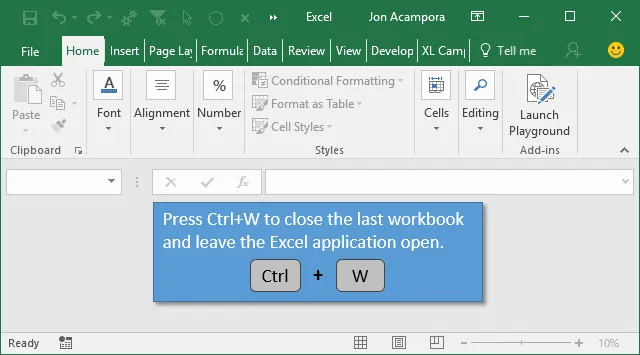
#12 – Close the Last Excel Workbook, But Leave Excel Open
In Excel 2013 for Windows the application changed to a Single Document Interface (SDI). That means we no longer have Excel workbooks open inside of one application window. Instead, we have one application window open per workbook.
When we close the last workbook we have open by pressing the “X” (close button) in the top-right corner of the application window, the entire Excel application closes.
Sometimes we don’t want this if we are working on an add-in, personal macro workbook, or just don’t want completely restart Excel.
To leave the application window open, press Ctrl+W on the keyboard to close the workbook only. This will close the workbook without closing the application window.
We can also add the Close Window button to the Quick Access Toolbar, to preform this operation with the mouse.
Bonus tip: Ctrl+W also works to close tabs in your web browser window.
Mac shortcut: Ctrl+W or Cmd+W works on the Mac version. The behavior of the SDI is a little different. The app window will close but the app will remain open in the task bar.
#13 – Create Keyboard Shortcuts for any Command with the Quick Access Toolbar
The Quick Access Toolbar (QAT) was introduced with the ribbon in Excel 2007, and allows us to create buttons for our most commonly used commands. This saves us from having to navigate through the tabs in the ribbon to find a button.
Each button in the QAT has a keyboard shortcut assigned to it.
1.With any cell or object selected, press and release the Alt key on the keyboard.
2.You will see numbers appear above the buttons on the QAT. These are the shortcuts to press the buttons.
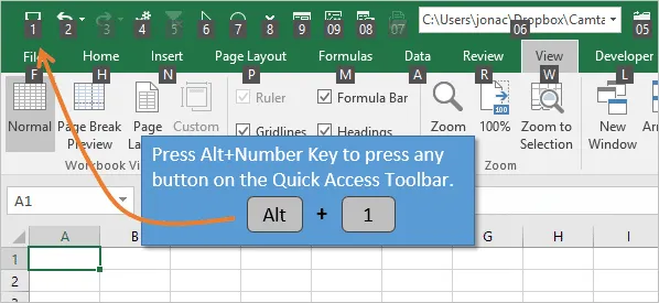
So Alt+1 is the keyboard shortcut to press the first button in the QAT. Put your favorite command in that position and you now have a keyboard shortcut for it. This is great for commands that don’t have dedicated keyboard shortcuts.
Mac shortcut: Unfortunately, the Mac version does not have the Alt shortcut keys for the QAT.
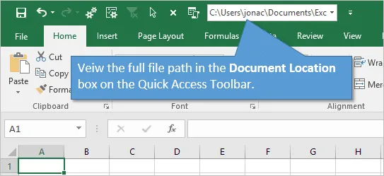
#14 – Add Document Location/File Path to the QAT
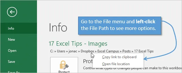
Sometimes when we have an Excel file open we want to quickly see which folder or drive the file is saved on. This is especially true if you are working with files on different servers or mapped drives.
We can add a box called the Document Location to the QAT to see the file path of the file that is currently open.
1.Right-click the ribbon or QAT and select “Customize the Quick Access Toolbar…”
2.In the drop-down menu in the top left of the Window select Commands Not in the Ribbon.
3.Scroll down in the list box below to find Document Location.
4.Double-click it to add it to the QAT and press OK.
You will now see the Document Location box in the QAT. This will appear every time you open Excel. It will also change every time you open or activate a different Excel file.
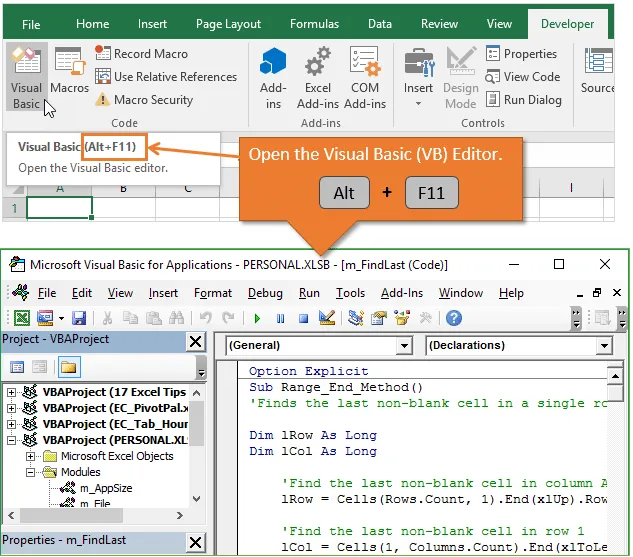
#15 – Open the Visual Basic Editor
The Visual Basic Editor (VB Editor) is the application where we write macros and create userforms. This application comes with Excel, and unlocks a whole new world of programming and automating Excel with VBA.
The keyboard shortcut to open the VB Editor is Alt+F11. We can also open the VB Editor by pressing the Visual Basic button on the Developer Tab of the ribbon. Once in the VB Editor, you can press Alt+F11 again to get back to Excel.
Mac shortcut: Unfortunately, the Mac does not have this shortcut key. The current VB Editor for the Mac 2016 version is pretty limited on it’s capabilities. Hopefully that will change in the future
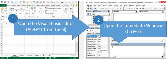
#16 – Open the VBA Immediate Window
The VBA Immediate window is an amazing tool that can help us with all kinds of tasks. We use it frequently when writing and debugging macros. But it can also be used to run one line of code or get some information about objects in the application.
To open the Immediate Window, press Alt+F11 to open the VB Editor, then press Ctrl+G to open the Immediate Window.
From here you can type a line of code and then press enter to run the code. A good example is removing the page break lines that appear after running print preview. You can type or copy/paste the following code into the Immediate Window, then hit Enter, to clear the page breaks lines.
ActiveSheet.DisplayPageBreaks = False
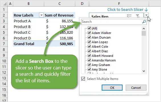
#17 – Add a Search Box to Your Slicers
Unfortunately, we can’t actually add a search box to our slicers. However, I created a bit of a workaround that gets the job done.
Thank For Reading This post