Hello its a me again! Today we continue with Mathematical Analysis getting into Differentiation Theorems and also some more in-depth examples! I suggest you to check out the Derivatives post if you haven't already! So, without further do let's get started!
Fundamental Differentiation Theorems:
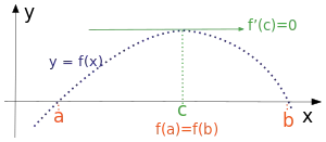
Fermat's Theorem:
Suppose a function f: A->R, that is differentiable at the global extremum (maxima or minima) point x0, that is an internal point of A. Then we know that f'(x0) = 0.
Rolle's Theorem:
Suppose a real function f that is continuous in the range [a, b] and differentiable in the range (a, b), where f(a) = f(b). Then we know that there is atleast one point x0 in (a, b) so that f'(x0) = 0.
Mean Value Theorem:
Suppose a real function f that is continuous in the range [a, b] and differentiable in the range (a, b). Then we know that there is atleast one point x0 in (a, b) so that f'(x0) = (f(b) - f(a)) / (b - a).
Fermat's theorem is simple to understand, cause whenever there is a global internal extremum and we plot the graph of this function we see that the tangent at this point has a slope/angle that is parallel to the x'x axis.
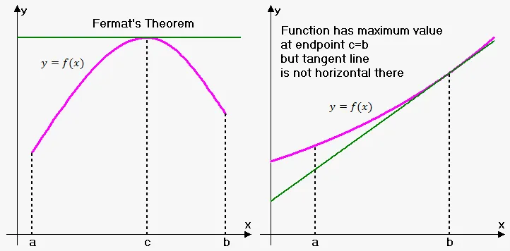
In this picture you can see that the left one does exactly what I said and the tangent is parallel to the x'x axis. But, for the right one we see that the global extremum was not internal (maximum was at the final point b of the range) and so the slope of the tangent there was not equal to 0 and therefore the tangent was not parallel and so Fermat's theorem doesn't apply here!
Rolle's theorem can be proven by using the Mean Value Theorem, cause when f(a) = f(b) there is at least one point so that f'(x0) = (0 - 0) / (b - a) = 0.
The last one can also be seen directly by plotting the graph of a function:

You can see that between two points there is always a point that has a tangent parallel to the line that we get when connecting the points a and b. There could also be more, but at least one is always there!
So, where do these help us? There is some stuff that we covered already that can now be calculated much more easily by using those Theorems instead of the actual definition and other things that took more time.
Derivatives as a tool of studying functions:
Monotony:
The monotony and slope of a function can be calculated by finding the first derivative's sign and value. So, when positive the function is increasing in that range and when it is negative the function is decreasing. The value of the derivative gives us information about the magnitude/amount of change.
Extrema:
The points where the value of the first derivative is zero are extrema.
This also means that:
- At such a point the monotony of the function changes (increasing to decreasing or vise versa)
- The type of extrema depends on the value of the second derivative at such a point x0. When f''(x0) > 0 then this point is a local minimum and when f''(x0) < 0 then this point is a local maximum.
The last one seems to be inverse, but it's actually the right way around, and we will get into examples later on so that you see why!
Set of range:
This set can be calculated from the endpoints, where we had extrema points and limit values to infinity (when they are inside of the domain of definition) or everywhere the function is undefined. From all those values we use the maximum and minimum value to specify the range f(A).
We will get into an example later on!
Curvature, convexity and concavity:
The points where the second derivative is equal to zero and the curvature changes are the so called turning points or inflection points. In such a point the function changes from convex to concave or vise versa. A function is convex where f''(x) > 0 and concave where f''(x) < 0. Convex means that the tangent line lies below the graph of the function and concave means that the tangent line lies above the graph of the function.
Asymptotes:
Lines that have a distance that approaches zero to the curve of a function as x or y or both coordinates approach infinity are the so called aymptotes of this function.
We have 3 types of asymptotes:
- Horizontal asymptotes
- Vertical asymptotes
- Oblique asymptotes
Let's get into how we find if they exist and also calculate them.
Horizontal asymptote:
Horizontal asymptotes are horizontal lines that the function graph approaches when x goes to +-∞, where ∞ needs to be in the definition set of the function.
The horizontal line y = a is a horizontal asymptote when:
lim x->+∞ (or -∞) f(x) = a, where a needs to be a real number and not ∞.
Vertical asymptote:
We have vertical asymptotes when the definition set of our function doesn't contain a point x0.
When at least one of the one-sided limits to x0 gives us +-∞ then the vertical line x = x0 is a vertical asymptote of our function.
Oblique asymptote:
When the definition set of our function contains +∞ or -∞ then we can also check for oblique asymptotes using the following equations:
lim x->+∞ (or -∞) [ f(x) / x] = a, where a is a real number.
lim x->+∞ (or -∞) [f(x) - a*x] = b, where b is a real number.
Then our function has a oblique asymptote with a line y = a*x + b.
D'Hospital's Rule:
Another useful rule that can be used for calculating limits is the so called D'Hospital Rule. When our limit is in an indeterminate form 0/0 or ∞/∞ we can use the following rule to calculate the limit to some x0 or even ∞. A limit is equal to the limit where we differentiate the numerator and denominator.
This looks like that:
lim x->x0 (or +-∞) [ f(x) / g(x)] = lim x->x0 (or +-∞) [ f'(x) / g'(x)]
This means that whenever we have a indeterminate form we will differentiate as many times as needed until the indeterminate form is gone.
Examples:
Find the definition set, monotony, extremas, set of range, curvature (convexity, concavity) and asymptotes of the following functions:
1. f(x) = x - xlnx
Because the function contains a logarithm lnx, we know that x > 0.
This means that the function is defined in (0, +∞) or the so called R+
Let's check out the monotony.
The first derivative is:
f'(x) = (x - xlnx)' = x' - (xlnx)' = 1 - [x'lnx + x(lnx)'] = 1 - lnx - x*(1/x) = -lnx.
When 0<x<1 we have that lnx<0 and so f'(x) > 0 and f is increasing
When x == 1 we have taht lnx == 0 and so f'(x) == 0 and x0 = 1 is a global extrema
When x>1 we have that lnx>0 and so f'(x) < 0 and f is decreasing
This means that x0 is a global maximum, cause f is inscreasing and then decreasing.
f(1) = 1 - 1*ln1 = 1 - 1*0 = 1 and so the set of range f(R+) = (-∞, 1)
Let's now get into the curvature.
f''(x) = [f'(x)] ' = (-lnx)' = -1/x.
x > 0 means that -1/x < 0 and so f''(x) < 0 and f is convex
-1/x is zero only when x = ∞ and so we don't have an inflection point.
Let's now check for asymptotes.
We already know that there is no vertical one, cause limx->0 f(x) = 0 that is not ∞
We can check for an oblique to take care of horizontal's as well.
lim x->∞ (f(x) / x) = lim x->∞ [x(1 - lnx) / x] = lim x->∞ (lnx - 1) = ∞
This means that we don't have any asympotes!
2. f(x) = 1/(1+x^2)
f(x) is defined in the whole real space R = (-∞, ∞) , cause the denominator is always non-zero.
To find the monotony we need the first derivative of f(x).
f'(x) = [1/(1+x^2)]' that needs the Reciprocal rule (special case of quotient)!
So, f'(x) = −(1+x^2)'/ (1+x^2)^2 = -2*x / (1+x^2)^2.
The denominator is a square and is always >= 0 and here always >0, cause 1 + x^2 >0.
When x > 0 => -2x < 0 => f'(x) < 0 and so f is decreasing
When x < 0 => -2x > 0 => f'(x) > 0 and so f is increasing
When x == 0 => f'(x) == 0 and so x0 = 0 is a extrema point.
Because, f(x) changes monotony from increasing to decreasing we know that x0 is a global maximum.
f(0) = 1 and so the set of range is f(R) = (0 , 1], cause f is non-zero and f(0) = 1 is the maxima.
Let's check out the curvature now.
f''(x) = [f'(x)]' = [-2*x / (1+x^2)^2]' that we can calculate using the Quotient Rule.
So, f''(x) = {(-2*x)'*(1+x^2)^2 -(-2*x)*[(1+x^2)^2]'} / (1+x^2)^4. Yeah!
f''(x) = {-2*(1+x^2)^2 + 2*x*[2*(1+x^2)*(1+x^2)']} / (1+x^2)^4. Well
f''(x) = {-2*(1+x^2)^2 + 2*x*2*(1+x^2)*2*x} / (1+x^2)^4. OK
f''(x) = [-2*(1+x^2)^2 + 8x^2(1+x^2)] / (1+x^2)^4. Hmm
If you see closely you can see that we can take 1+x^2 as a common pair on the numerator.
f''(x) = [(1+x^2)*(-2 - 2x^2 + 8x^2)] / (1+x^2)^4 and so
f''(x) = (6x^2 - 2) / (1+x^2)^3. Finally done
The denominator is again always positive, cause 1 + x^2 > 0.
The numerator 6x^2 - 2 = 0 when x^2 = 2/6 = 1/3
And so x = +- root(1/3) = +- root(3/9) = +- root(3) / 3 are the inflection points.
Let's check the curvature at all the ranges.
When x < -root(3) / 3 for example -1 we have that:
6x^2 - 2 = 6 - 2 = 4 > 0 and so f''(x) > 0 and f is concave.
When -root(3) / 3 < x < root(3)/3 for example 0 we have that:
6x^2 - 2 = -2 < 0 and so f''(x) < 0 and f is convex.
When x > root(3) / 3 for example 1 we have that:
6x^2 - 2 = 6 - 2 = 4 > 0 and so f''(x) > 0 and f is concave.
Let's now lastly check for asymptotes.
The function f has no vertical asymptotes, because the domain of definition is equal to R.
lim x->+-∞ f(x) = lim x->+-∞ [1/(1+x^2)] = 1/+-∞ = 0 that is a real number
This means that f has a horizontal asymptote y = 0.
lim x->+-∞ (f(x) / x) = lim x->+-∞ [x/(1+x^2)] it goes up when divided
We have a indeterminant form ∞/∞ and so we use the D'hospital rule and get:
lim x->+-∞[1/2x] = 1/+-∞ = 0 = a, that is a real number.
Let's also check the second condition.
lim x->+-∞[f(x) - a*x] = limx->+-∞ f(x) = o that we already calculated previously.
So, we ended up with the same horizontal asymptote y = 0 and f has no oblique asymptote.
And this is it for today and I hope that you enjoyed it!
From next time on we will start talking about Integrals!
Bye!