
Hello it's a me again drifter1! Today we continue with Linear Algebra getting into how we solve Linear Systems using the Gauss Method. I will first give you some theory that we need and then get into how we apply the Gauss method. So, without further do, let's get straight into it!
Linear System Representation:
A Linear System contains 2 or more Linear Equations that contain 1, 2, ... n variables. Each linear equation will contain some or all of those common variables that will be multiplied by some coefficients.
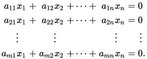
So, an Linear System looks like this:
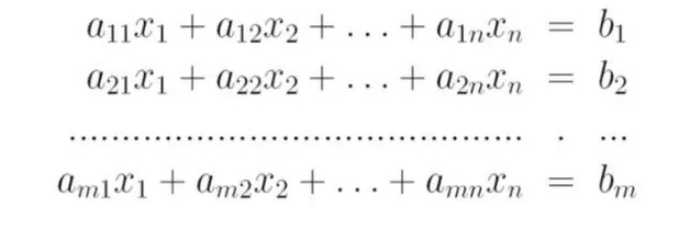
Where:
- aij are the coefficients
- x1, x2, ..., xn are the variables
- b1, b2, ... bm are the constants of the equations
Matrix form:
We can create a matrix that contains all the coefficients. This matrix looks like this:
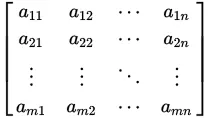 Coefficient matrix
We can also create two column-vectors, where one contains only the variables and the other only the constants of the linear system. Those two will be called x and b and so our Linear System will now be a multiplication between A and x that gives us b!
This looks like this:

Another important matrix is called the Augmented matrix that contains matrix A and b, having b be added to the end of matrix A.
So, an Augmented matrix A/b looks like this:
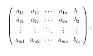
This last matrix will help us in the Gaussian Elimination method!
Example:
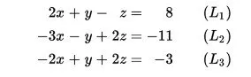
Suppose we have a linear system like this one:
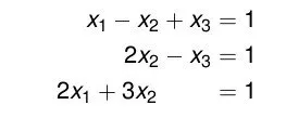
The matrix representation of the same system is:
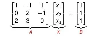
You should be very careful when putting the coefficients in the A matrix, cause in your system the order may not be right. Each column needs to contain the coeffiecients of a specific variable and when we don't have one we will have to put 0!
Linear System Solutions:
A linear system can have 3 possible outcomes:
- One unique solution that contains a value for each of the n variables (Intersecting lines)
- Infinite solution combinations of those n variables (Coincident lines)
- No solutions (Parallel lines)
An combination of values for the n variables that verifies all the linear equations of the linear system at the same time is called a solution.
Homogeneous Linear System:
A homogeneous linear system is a special case where the b matrix is a zero-column matrix and has only 0. This special linear system has always a solution, the all-zero solution, and so can either have one unique solution that is the all-zero solution or has infinite solutions if we find another one that is different to the all-zero solution.
Such a linear system looks like this:
Matrix Elementary Operations:
After talking about the matrix representation we can now start talking about how we can make changes to it. This can be done using some elementary operations that actually are simple operations between rows or columns.
We can do the following elementary operations:
- Row/Column switching, where we switch the places of 2 rows or columns and note it as ri<->rj or ci<->cj having i and j be the indexes of the rows/columns in the matrix
- Row/Column multiplication, where we multiply a whole row or column by a non-zero constant and note it as ri<->a*ri or ci<->a*ci having i be the index of the row/column and a!=0
- Row/Column addition, where we replace a row/column with the sum of this row/column with another row/column. The other row/column can be multiplied by a non-zero constant and so the noting is ri <-> ri +a*rj or ci <-> ci + a*cj having i and j be the indexes of the rows/columns and a!=0
The matrix that we get after doing elementary operations is called an elementary matrix and this matrix is equivalent to the matrix we started with. So, 2 matrixes are called equivalent when one is the result of elementary operations on the other matrix. Using those operations we can "simplify" our matrix.
Echelon/Canonical Forms:
In the Gaussian method we talk about row/column (reduced) echelon forms of a given matrix. We will get each of those types depending on if we did elementary operations on the rows or columns.
A matrix is an row echelon form when:
- All nonzero rows are above any rows of all zeroes
- The leading coefficient (pivot) of a nonzero row is always strictly to the right of the leading coefficient of the row above it
Such a matrix looks like this:
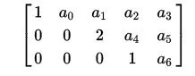
This means that we order the rows, having the rows with "more" non-zero coefficients be on top of the ones without. Zero-rows will be on the bottom of the matrix.
A matrix is in a form called row canonical form when:
- It is in row echelon form
- The pivot is '1' and is the only nonzero entry in its column
Such a matrix looks like this:
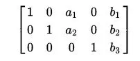
You can see that the rules of the row echelon form are still true, but the coefficient of each row is '1' and is also the only nonzero coefficient of it's column. This second form is also unique for each linear system.
These exact form will lead us to how we solve a linear system using the Gauss Method.
Gaussian Elimination Method:
The Gauss Method uses the Matrix Representation of A*x = b and starts doing elementary operations on the augmented A/b matrix until we end up with an canonical form!
So, the steps of the Gaussian method are:
- Create the augmented A/b matrix
- Do elementary operations between the rows until you get a canonical form (we will get into how we get this form in a sec.)
- Write down each linear equation starting out from the bottom and the first nonzero row and start solving the variables. What you get in the end will be the solution (you might also get infinite or no solutions as I told you earlier)
Getting the canonical form:
The most essential step of the Gaussian method is how we get the canonical form. It's actually not so difficult, but you will have to follow some specific steps.
Steps:
- Select the row of the matrix that has the first nonzero element in the most-left column and move it to the top if it's not.
- Do a row multiplication on this same row with an appropriate constant that changes the first nonzero element to '1' and makes it a pivot.
- We substract the other rows with appropriate multiplications of the first row, so that all the other elements of the column the pivot is in are '0', and the pivot is the only nonzero element of it's column.
- We repeat steps 1, 2, 3 on the other rows, so that all rows have pivots. That way our matrix will be in row echelon form.
- Lastly we also put zeros on top of the pivots so that we end up with an canonical form. For that matter we start from the last nonzero row and make the values on top of the pivot's row (in the row on top) to '0'. We continue this process on the other higher rows until our matrix is in canonical form.
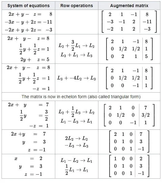
You can stop after reaching step 4, cause this is the Gauss Method. If you continue getting into step 5 and get up to the canonical form the method will be called Gauss-Jordan. But, we mostly tend to simply call it Gauss!
In wikipedia there is a nice full-on example where you can see this steps in action.
And this is actually it and I hope you enjoyed it!
Next time we will get into how we solve a square system using determinants.
Bye!