[Image1]
Introduction
Hey it's a me again @drifter1!
Today we continue with my mathematics series about Signals and Systems in order to cover Exercises on Modulation.
So, without further ado, let's dive straight into it!
Modulation Recap
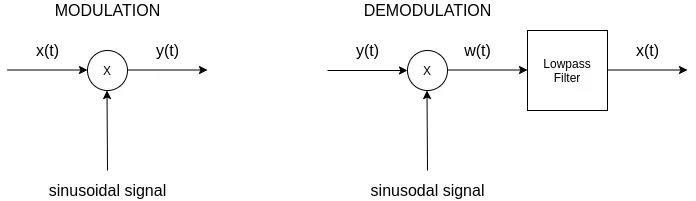
Let's first refresh our knowledge on the concept of modulation.
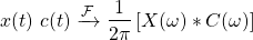
Modulation is one of the quite useful properties of the Fourier Transform, which tells us that the FT of two signals which get multiplied in the Time-Domain is turned into a convolution of their individual FTs whilst in the Frequency-Domain.
If we consider x(t) (or x[n]) to be the signal to be "modulated", and c(t) (or c[n]) to be the signal that modulates it, or otherwise known as the carrier signal, we can specify the following:
In continuous-time systems and signals, the two basic modulation techniques are:
- Amplitude Modulation (AM) = Transmission in the Frequency of the Carrier Signal
- Frequency Modulation (FM) = Transmission in the Amplitude of the Carrier Signal
On the other hand, in the case of discrete-time, modulation is most commonly used in the case of modern, digital communication systems. One great example of this is Time-Division Multiplexing (TDM), where amplitude modulation with time-shifted pulse carriers can be used to transfer multiple signals (and so multiple data) using the same pulse carrier.
Continuous-Time Modulation Example (Based on 13.1 from Ref1)
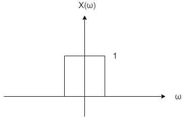
Let's consider an continuous-time amplitude modulation system with input x(t) as shown below:

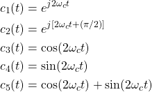
Determine the Fourier Transform of the output (only the magnitude), Y(ω), for each of the following carriers:
Solution
The Fourier Transform of the sinc function is a rectangular pulse, and as such the graph of X(ω) is:
For the first carrier its possible to use the shifting property of the Fourier Transform, which gives us:
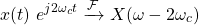
And so Y(ω) can be plotted as follows:
For the second carrier we take the result of the previous case and multiply by e jπ/2, which gives us:

Of course this is the phase-shifting property and so the magnitude remains unaffected.
Next up are the sinusoidal carriers.
The cosinus signal can be split into two complex exponentials, which makes the modulation a sum of two values:

The resulting plot is the following:

Similar to the first and second carrier, the third and fourth carrier also give us the same magnitude, but with a different phase spectrum.
So, let's only split the sinus signal into the two complex exponentials:

The fifth and final carrier is a combination of the previous two sinusoidal signals, and so the 1 / 2 scaling of the magnitude of both cases gets undone, giving us the following graph:

The phase spectrum analysis gets quite complicated for this case, and so let's again skip it.
Discrete-Time Modulation Example (Based on 15.2 from Ref1)
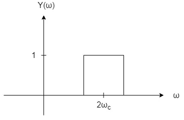
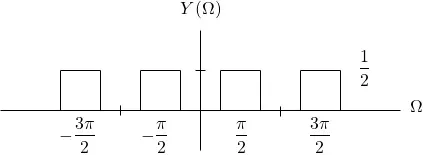
Let's consider an discrete-time modulation system with an sinusoidal carrier signal, c[n] = cos[Ω0 n], and the following input:
Sketch the output, Y(Ω), for Ω0 = π / 2.
Solution
The Fourier Transform of the sinusodial carrier leads to the following impulses:

As such, based on the modulation theorem (or property), X(Ω) will be centered around each impulse of C(Ω) and scaled by 1 / 2.
This results in the following graph:
RESOURCES:
References
Images

Mathematical equations used in this article were made using quicklatex.
Block diagrams and other visualizations were made using draw.io and GeoGebra
Previous articles of the series
Basics
- Introduction → Signals, Systems
- Signal Basics → Signal Categorization, Basic Signal Types
- Signal Operations with Examples → Amplitude and Time Operations, Examples
- System Classification with Examples → System Classifications and Properties, Examples
- Sinusoidal and Complex Exponential Signals → Sinusoidal and Exponential Signals in Continuous and Discrete Time
LTI Systems and Convolution
- LTI System Response and Convolution → Linear System Interconnection (Cascade, Parallel, Feedback), Delayed Impulses, Convolution Sum and Integral
- LTI Convolution Properties → Commutative, Associative and Distributive Properties of LTI Convolution
- System Representation in Discrete-Time using Difference Equations → Linear Constant-Coefficient Difference Equations, Block Diagram Representation (Direct Form I and II)
- System Representation in Continuous-Time using Differential Equations → Linear Constant-Coefficient Differential Equations, Block Diagram Representation (Direct Form I and II)
- Exercises on LTI System Properties → Superposition, Impulse Response and System Classification Examples
- Exercise on Convolution → Discrete-Time Convolution Example with the help of visualizations
- Exercises on System Representation using Difference Equations → Simple Block Diagram to LCCDE Example, Direct Form I, II and LCCDE Example
- Exercises on System Representation using Differential Equations → Equation to Block Diagram Example, Direct Form I to Equation Example
Fourier Series and Transform
- Continuous-Time Periodic Signals & Fourier Series → Input Decomposition, Fourier Series, Analysis and Synthesis
- Continuous-Time Aperiodic Signals & Fourier Transform → Aperiodic Signals, Envelope Representation, Fourier and Inverse Fourier Transforms, Fourier Transform for Periodic Signals
- Continuous-Time Fourier Transform Properties → Linearity, Time-Shifting (Translation), Conjugate Symmetry, Time and Frequency Scaling, Duality, Differentiation and Integration, Parseval's Relation, Convolution and Multiplication Properties
- Discrete-Time Fourier Series & Transform → Getting into Discrete-Time, Fourier Series and Transform, Synthesis and Analysis Equations
- Discrete-Time Fourier Transform Properties → Differences with Continuous-Time, Periodicity, Linearity, Time and Frequency Shifting, Conjugate Summetry, Differencing and Accumulation, Time Reversal and Expansion, Differentation in Frequency, Convolution and Multiplication, Dualities
- Exercises on Continuous-Time Fourier Series → Fourier Series Coefficients Calculation from Signal Equation, Signal Graph
- Exercises on Continuous-Time Fourier Transform → Fourier Transform from Signal Graph and Equation, Output of LTI System
- Exercises on Discrete-Time Fourier Series and Transform → Fourier Series Coefficient, Fourier Transform Calculation and LTI System Output
Filtering, Sampling, Modulation, Interpolation
- Filtering → Convolution Property, Ideal Filters, Series R-C Circuit and Moving Average Filter Approximations
- Continuous-Time Modulation → Getting into Modulation, AM and FM, Demodulation
- Discrete-Time Modulation → Applications, Carriers, Modulation/Demodulation, Time-Division Multiplexing
- Sampling → Sampling Theorem, Sampling, Reconstruction and Aliasing
- Interpolation → Reconstruction Procedure, Interpolation (Band-limited, Zero-order hold, First-order hold)
- Processing Continuous-Time Signals as Discrete-Time Signals → C/D and D/C Conversion, Discrete-Time Processing
- Discrete-Time Sampling → Discrete-Time (or Frequency Domain) Sampling, Downsampling / Decimation, Upsampling
- Exercises on Filtering → Filter Properties, Type and Output
Final words | Next up
And this is actually it for today's post!
Next time we will get into Sampling and Interpolation examples...
See Ya!

Keep on drifting!