[Image1]
Introduction
Hey it's a me again @drifter1!
Today we continue with my mathematics series about Signals and Systems in order to cover Exercises on Discrete-Time Fourier Series and Transform.
So, without further ado, let's dive straight into it!
Discrete-Time Fourier Series Coefficients Calculation [Based on 10.3 from Ref1]
Let's consider the following periodic sequence:

Find the appropriate expression for the envelope of the Fourier series coefficients and sample it.
Solution
In discrete-time an orthogonal pulse in the range [-N1, N1] can be represented as follows:

Using complex exponentials, the Fourier series coefficient is thus given as follows:

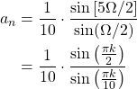
As such, the samples can be taken from the sampling function, which leads us to the following envelope:

In the case of this example, N1 = 2, and N = 10, and so:
Discrete-Time Fourier Transform Calculation [Based on 11.1 from Ref1]
Compute the discrete-time Fourier transform of the following signals:


Solution
The Fourier transform can be easily calculated with the help of Fourier transform pair tables and properties that we discussed throughout the series of articles.
a.
The first case is a slighly different representation of one of the known Fourier transform pairs, which is:

For |a| > 1, this can be re-written as:
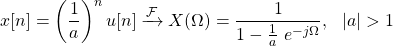
Thus, for a = 6, which is the first signal, the result is:

b.
This case is quite similar to the first one.
Let's start re-formulating in order to achieve such a form:

From the previous example we know that:

Due to linearity its possible to multiply both sides by 36, which yields:

From the time-shifting property, we then get the final result:

c.
The orthogonal pulse can be easily described using unit step functions, in the following manner:

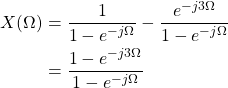
The Fourier transform of the unit step function is:

And time-shifting by 3 leads to the following result:

So, the final result is:
Output of LTI System [Based on 11.2 from Ref1]
The following linear constant-coefficient difference equation describes an LTI system initially at rest:

Using Fourier transforms, let's evaluate y[n] for each of the following inputs:

Solution
First of all, let's take the Fourier transform of both sides of the LCCDE:

As such H(Ω) is equal to:

a.
For x[n] = δ[n], X(Ω) = 1, which makes the output equal to the impulse response:

and, so the Inverse Fourier Transform gives us the output y[n] and h[n] in the same time:

b.
The Fourier Transform of x2[n] is:

and so the output Y(Ω) is equal to:

Taking the Inverse Fourier Transform gives us the final result:

RESOURCES:
References
Images

Mathematical equations used in this article were made using quicklatex.
Block diagrams and other visualizations were made using draw.io and GeoGebra
Previous articles of the series
Basics
- Introduction → Signals, Systems
- Signal Basics → Signal Categorization, Basic Signal Types
- Signal Operations with Examples → Amplitude and Time Operations, Examples
- System Classification with Examples → System Classifications and Properties, Examples
- Sinusoidal and Complex Exponential Signals → Sinusoidal and Exponential Signals in Continuous and Discrete Time
LTI Systems and Convolution
- LTI System Response and Convolution → Linear System Interconnection (Cascade, Parallel, Feedback), Delayed Impulses, Convolution Sum and Integral
- LTI Convolution Properties → Commutative, Associative and Distributive Properties of LTI Convolution
- System Representation in Discrete-Time using Difference Equations → Linear Constant-Coefficient Difference Equations, Block Diagram Representation (Direct Form I and II)
- System Representation in Continuous-Time using Differential Equations → Linear Constant-Coefficient Differential Equations, Block Diagram Representation (Direct Form I and II)
- Exercises on LTI System Properties → Superposition, Impulse Response and System Classification Examples
- Exercise on Convolution → Discrete-Time Convolution Example with the help of visualizations
- Exercises on System Representation using Difference Equations → Simple Block Diagram to LCCDE Example, Direct Form I, II and LCCDE Example
- Exercises on System Representation using Differential Equations → Equation to Block Diagram Example, Direct Form I to Equation Example
Fourier Series and Transform
- Continuous-Time Periodic Signals & Fourier Series → Input Decomposition, Fourier Series, Analysis and Synthesis
- Continuous-Time Aperiodic Signals & Fourier Transform → Aperiodic Signals, Envelope Representation, Fourier and Inverse Fourier Transforms, Fourier Transform for Periodic Signals
- Continuous-Time Fourier Transform Properties → Linearity, Time-Shifting (Translation), Conjugate Symmetry, Time and Frequency Scaling, Duality, Differentiation and Integration, Parseval's Relation, Convolution and Multiplication Properties
- Discrete-Time Fourier Series & Transform → Getting into Discrete-Time, Fourier Series and Transform, Synthesis and Analysis Equations
- Discrete-Time Fourier Transform Properties → Differences with Continuous-Time, Periodicity, Linearity, Time and Frequency Shifting, Conjugate Summetry, Differencing and Accumulation, Time Reversal and Expansion, Differentation in Frequency, Convolution and Multiplication, Dualities
- Exercises on Continuous-Time Fourier Series → Fourier Series Coefficients Calculation from Signal Equation, Signal Graph
- Exercises on Continuous-Time Fourier Transform → Fourier Transform from Signal Graph and Equation, Output of LTI System
Final words | Next up
And this is actually it for today's post!
From next time we will start getting into concepts like Filtering, Modulation, Sampling, Interpolation etc.
See Ya!

Keep on drifting!