[Image1]
Introduction
Hey it's a me again @drifter1!
Today we continue with my mathematics series about Signals and Systems in order to cover Exercise on Convolution.
So, without further ado, let's dive straight into it!
Discrete-Time Convolution Example [Based on P4.2 from Ref1]
Let's determine the discrete-time convolution of the following two signals:
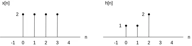
Solution
The convolution sum that we want to calculate is defined as:

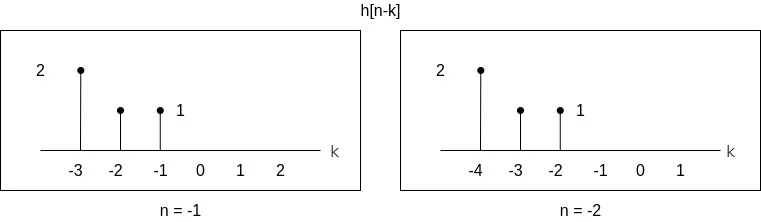
Its easy to notice that the convolution sum requires an reflected version of h[n].
Reflecting h[n] about the origin and changing the unit from n to k leads to h[-k]:

which is basically h[n - k] for n = 0.
For the values n < 0 time-shifting leads to values of h[n - k] which result to zero contribution to the convolution sum.
More specifically, the resulting h[n - k] are not in the closed range [0, 3] in which x[k] is non-zero.
For example n = -1 and n = -2:
As such, the sums that need to be calculated start at n = 0, which leads us to the question: "When do we stop?".
Let's start increasing n, which will of course lead to a shifting of h[n - k] to the right by 1, 2, 3 etc.
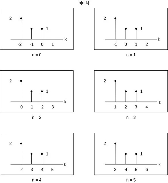
After n = 5 the graph of h[n - k] again contributes zero to the convolution sum. Therefore, the convolution can be easily calculated by using n in the range [0, 5], which leads to a result, y[n], of length 6.
Generally, the result is equal to the sum of the lengths of the individual discrete-time signal sequences x[n] and h[n] minus 1:

So, how do we get the final result? Well, its simply multiplying x[k] by the various shifts of h[n - k] and summing up those values. The result of this sum is then the value of the convolution y[n] for each specific point in time.
The values n = 0 and n = 1 give us:

which give us the values of the convolution y[n]:

Similarly, for the values n = 2 and n = 3 we have:

which gives us two 8 's.
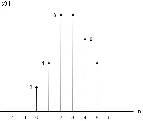
Lastly, for the values n = 4 and n = 5:

and so the convolution contributions 6 and 4, respectively.
Finally, the convolution between x[n] and h[n], which is y[n], can be now visualized as follows:
RESOURCES:
References
Images

Mathematical equations used in this article were made using quicklatex.
Block diagrams and other visualizations were made using draw.io
Previous articles of the series
Basics
- Introduction → Signals, Systems
- Signal Basics → Signal Categorization, Basic Signal Types
- Signal Operations with Examples → Amplitude and Time Operations, Examples
- System Classification with Examples → System Classifications and Properties, Examples
- Sinusoidal and Complex Exponential Signals → Sinusoidal and Exponential Signals in Continuous and Discrete Time
LTI Systems and Convolution
- LTI System Response and Convolution → Linear System Interconnection (Cascade, Parallel, Feedback), Delayed Impulses, Convolution Sum and Integral
- LTI Convolution Properties → Commutative, Associative and Distributive Properties of LTI Convolution
- System Representation in Discrete-Time using Difference Equations → Linear Constant-Coefficient Difference Equations, Block Diagram Representation (Direct Form I and II)
- System Representation in Continuous-Time using Differential Equations → Linear Constant-Coefficient Differential Equations, Block Diagram Representation (Direct Form I and II)
- Exercises on LTI System Properties → Superposition, Impulse Response and System Classification Examples
Fourier Series and Transform
- Continuous-Time Periodic Signals & Fourier Series → Input Decomposition, Fourier Series, Analysis and Synthesis
- Continuous-Time Aperiodic Signals & Fourier Transform → Aperiodic Signals, Envelope Representation, Fourier and Inverse Fourier Transforms, Fourier Transform for Periodic Signals
- Continuous-Time Fourier Transform Properties → Linearity, Time-Shifting (Translation), Conjugate Symmetry, Time and Frequency Scaling, Duality, Differentiation and Integration, Parseval's Relation, Convolution and Multiplication Properties
- Discrete-Time Fourier Series & Transform → Getting into Discrete-Time, Fourier Series and Transform, Synthesis and Analysis Equations
- Discrete-Time Fourier Transform Properties → Differences with Continuous-Time, Periodicity, Linearity, Time and Frequency Shifting, Conjugate Summetry, Differencing and Accumulation, Time Reversal and Expansion, Differentation in Frequency, Convolution and Multiplication, Dualities
Final words | Next up
And this is actually it for today's post!
Next time we will get into exercises on other topics that we covered!
See Ya!

Keep on drifting!