[Image1]
Introduction
Hey it's a me again @drifter1!
Today we continue with my mathematics series about Signals and Systems in order to cover Discrete-Time Modulation.
So, without further ado, let's dive straight into it!
Modulation in Discrete-Time
After covering continuous-time modulation, its now time for discrete-time modulation. Mulation is again a property of the Fourier Transform. Its the Fourier Transform of the multiplication/product of two signals, which turns into a convolution of their individual Fourier Transforms.
Consider x[n] to be the discrete-time signal to be "modulated".
The signal c[n] which is used to modulate x[n] is known as the carrier signal.
As a result, the modulation property can be written as:

The discrete-time Fourier Transform is a periodic function of frequency, which in turn makes the convolution also periodic. This is also the main difference with the continuous-time FT, where the convolution is linear.
Applications of Discrete-Time Modulation
The mathematics might seem similar, but the applications are different. As we saw last time, continuous-time modulation is a major concept of communication systems, as it is used for transmitting signals over various types of channels. But, in modern communication systems, these signals might have to go through a lot of stages and types of modulation. Thus, this conversion from modulation to another is better implemented digitally, with digital meaning discrete-time signals.
Discrete-time modulation is also useful in Filtering as it can be used to implement filters with a variable center frequency. Although it might be simpler to implement a fixed filter (in either continous- or discrete-time) and then use modulation to shift the signal spectrum in relation to the fixed filter center frequency.
Sinusoidal and Complex Expnential Carriers
Similar to continuous-time, the carrier signals in discrete-time can also be complex exponentials or sinusoidals.
The Fourier transform of an complex exponential signal is:
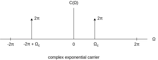
whilst the sinusoidal signal has a FT of:

A sinusoidal signal can easily be defined with the use of complex exponentials, as follows:

which also explains why the two graphical representations are so similar.
Pulse Carrier
Due to the nature of discrete samples, another useful type of carrier is also a periodic pulse, which is constant for some samples of the period and zero for the remainder.
This signal can then be used in modulation to extract time slices of the modulating signal.
Visually, pulse carriers look as follows:

The pulse train with the smallest time of being "on" can easily correspond to a periodic train of impulses, or even unit samples. A impulse train carrier allows sampling the modulating input signal, and leads to another very important concept, known as the sampling theorem. We will get into sampling in the next part of the series, but let's just note that it provides a major bridge between continuous-time and discrete-time systems and signals.
Pulse carriers can be useful in both continuous-time and discrete-time applications.
In continuous-time amplitude modulation with a pulse carrier, this leads to interesting results, such as:

Using this pulse carrier only specific time slices of the original signal x(t) are allowed to pass to the output y(t).
Modulation and Demodulation
Similar to continuous-time, when using sinusoidal carriers demodulation is defined as a modulation with a sinusoidal followed by a low-pass filter.

Complex exponentials just require a re-modulation in order to recover the original signal.
Let's also mention that modulating a signal with the signal (-1)n, passing it through a low-pass filter and re-modulating it again, is an easy way of implementing a high-pass filter:

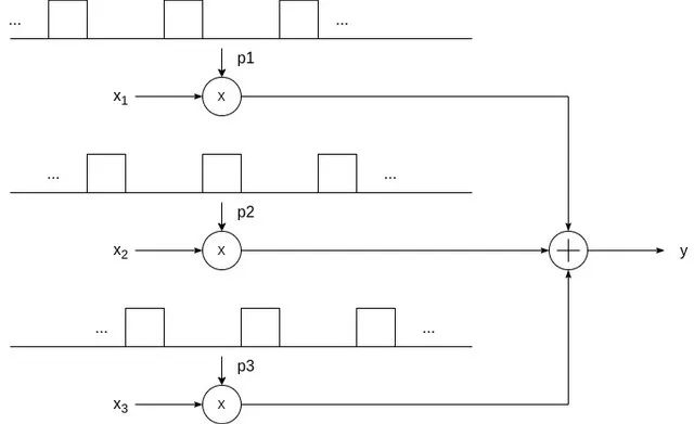
Time-Division Multiplexing
When representing the data for transmission, using pulse trains allows a specific type of multiplexing known as time-division multiplexing. Using TDM, the time slices from signals in other channels can be inserted to the carrier as well. Recovery or demodulation is also quite simple.
Visually, using amplitude modulation with a pulse carrier, multiple signals (and so multiple data) can be multiplexed through TDM, as follows:
RESOURCES:
References
Images

Mathematical equations used in this article were made using quicklatex.
Block diagrams and other visualizations were made using draw.io and GeoGebra
Previous articles of the series
Basics
- Introduction → Signals, Systems
- Signal Basics → Signal Categorization, Basic Signal Types
- Signal Operations with Examples → Amplitude and Time Operations, Examples
- System Classification with Examples → System Classifications and Properties, Examples
- Sinusoidal and Complex Exponential Signals → Sinusoidal and Exponential Signals in Continuous and Discrete Time
LTI Systems and Convolution
- LTI System Response and Convolution → Linear System Interconnection (Cascade, Parallel, Feedback), Delayed Impulses, Convolution Sum and Integral
- LTI Convolution Properties → Commutative, Associative and Distributive Properties of LTI Convolution
- System Representation in Discrete-Time using Difference Equations → Linear Constant-Coefficient Difference Equations, Block Diagram Representation (Direct Form I and II)
- System Representation in Continuous-Time using Differential Equations → Linear Constant-Coefficient Differential Equations, Block Diagram Representation (Direct Form I and II)
- Exercises on LTI System Properties → Superposition, Impulse Response and System Classification Examples
- Exercise on Convolution → Discrete-Time Convolution Example with the help of visualizations
- Exercises on System Representation using Difference Equations → Simple Block Diagram to LCCDE Example, Direct Form I, II and LCCDE Example
- Exercises on System Representation using Differential Equations → Equation to Block Diagram Example, Direct Form I to Equation Example
Fourier Series and Transform
- Continuous-Time Periodic Signals & Fourier Series → Input Decomposition, Fourier Series, Analysis and Synthesis
- Continuous-Time Aperiodic Signals & Fourier Transform → Aperiodic Signals, Envelope Representation, Fourier and Inverse Fourier Transforms, Fourier Transform for Periodic Signals
- Continuous-Time Fourier Transform Properties → Linearity, Time-Shifting (Translation), Conjugate Symmetry, Time and Frequency Scaling, Duality, Differentiation and Integration, Parseval's Relation, Convolution and Multiplication Properties
- Discrete-Time Fourier Series & Transform → Getting into Discrete-Time, Fourier Series and Transform, Synthesis and Analysis Equations
- Discrete-Time Fourier Transform Properties → Differences with Continuous-Time, Periodicity, Linearity, Time and Frequency Shifting, Conjugate Summetry, Differencing and Accumulation, Time Reversal and Expansion, Differentation in Frequency, Convolution and Multiplication, Dualities
- Exercises on Continuous-Time Fourier Series → Fourier Series Coefficients Calculation from Signal Equation, Signal Graph
- Exercises on Continuous-Time Fourier Transform → Fourier Transform from Signal Graph and Equation, Output of LTI System
- Exercises on Discrete-Time Fourier Series and Transform → Fourier Series Coefficient, Fourier Transform Calculation and LTI System Output
Filtering, Sampling, Modulation, Interpolation
- Filtering → Convolution Property, Ideal Filters, Series R-C Circuit and Moving Average Filter Approximations
- Continuous-Time Modulation → Getting into Modulation, AM and FM, Demodulation
Final words | Next up
And this is actually it for today's post!
Next time we will get into Sampling...
See Ya!

Keep on drifting!