My apologies for having been inactive for most of the last month - this was mainly a result of real life commitments catching up with me. Most significantly, I am rapidly moving towards the end of my PhD and there is still so much work I want to do - most of it a pipe dream I will never have the time for. That being said, I have made significant progress in discretely packaging simulations of my lab's brain model, with the ultimate goal of setting up a BOINC server for our lab.

For those that don't know me yet, my PhD is focussed on modelling the cells in the brain to such a level of detail that we can simulate brain function digitally. In my specific case, this allows me to observe the effects of neurodegenerative diseases such as Alzheimer's Disease to enable and advance drug development. The primary problem I encounter here is insufficient access to compute power to simulate my models to a satisfactory level of detail. BOINC will hopefully solve that limitation.
Unfortunately, no solution is perfect, and BOINC is not well suited to simulations that step through more than one dimension - in my case through space and time. In space, I model the smallest functional unit of the brain, and then connect them all together into what is called a space filling H tree, like below. Each dot is a single instance of the model. If that was the entire compute problem, I could easily cut the domain up into small pieces and wrap them in Docker wrappers to generate BOINC work units.

The problem arises when trying to step through time. Before the model can move forward in time, each node in space needs to exchange data with its nearest neighbours regarding ionic fluxes, blood volume, etc. In other words, all work at time t=1 needs to be completed before the simulation can progress to time t=2. Given that one simulation takes on the order of 100 million time steps, sending out 100 million tiny work batches, each of which needs to be returned in full before the next can be sent, is not a feasible solution.
To remedy the situation, I have attempted to vastly increase the size of the timesteps used in the simulation. This results in significant loss of accuracy, but that can be counteracted by careful interpolation to predict the behaviour between timesteps that were not explicitly simulated. What this means is that instead of stepping from t=1 to t=2 to t=3, we can step from t=1 to t=10 to t=20. Until recently the performance of large timestepping was not satisfactory, but we have just achieved successful replication of experimental BOLD data using the new implementation.
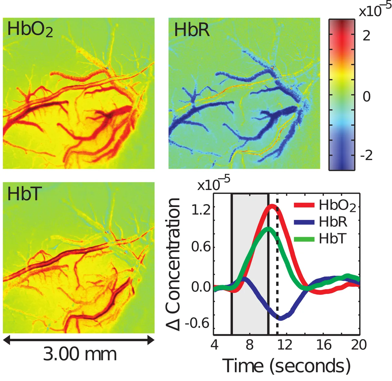
Allow me to begin by introducing the experimental data, which requires a little background knowledge. Your blood contains hemoglobin, which is used to carry oxygen to the cells that need it. Oxyhemoglobin (HbO2) is carrying oxygen, while deoxyhemoglobin (HbR) has deposited its oxygen where it is needed and is returning to the lungs to get more. We often refer to the total hemoglobin in the blood as HbT.
What you are seeing below is the cerebral vasculature of a rat after the region of the brain being observed is stimulated. I will not go into detail, as it's not pleasant how these experiments are done, and they are not done by my lab. The key thing to notice is that as a result of stimulation the blood vessels of the rat dilate (get wider), resulting in more oxyhemoglobin arriving at the active cells, which also increases the total hemoglobin present. Meanwhile, due to the significantly increased bloodflow, the deoxyhemoglobin is flushed out rapidly to return to the lungs. The time series in the bottom right shows the average behaviour observed in each of the other 3 fields over time. Note the rise in deoxyhemoglobin and drop in oxyhemoglobin at the very start of stimulation before the system corrects, which has not been simulated accurately before.
We attempted to replicate this data using our homegenous model with large timesteps, resulting in the image below. Due to our model not capturing individual blood vessels, but the aggregate response, the first three images will look different. The time series of the aggregate behaviour is the key point of note:
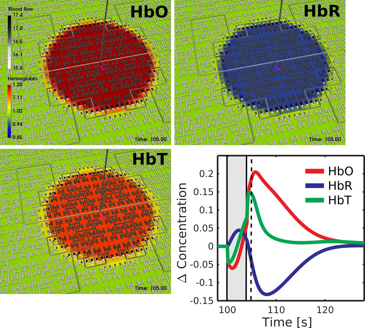
Not only were we able to accurately replicate the governing behaviour of the response, but we also replicated the transient dip observed at the very start of stimulation. I can imagine this does not excite any of you nearly as much as it does me, but this brings us significantly closer to encapsulating our model in a BOINC project, which in turn brings us closer to addressing neuro-degenerative diseases afflicting our elderly.
While you are not yet able to contribute to my project, there are already many other projects that can use your help! You can advance their work by donating the idle cycles of your computer, phone, tablet, you name it to the cause. Applications cover the fields of mathematics, medicine and astrophysics, allowing you to help do anything from mapping the Milky Way to developing drugs for cancer patients. To get started, you can get set up with BOINC here.
Just like Steemit rewards content creators for their work in the cryptocurrency STEEM, you can be rewarded for the research you contribute through BOINC in GRC. If you would like to be reimbursed for your contribution to academia, you can get started here.