Warning:
This post is quite technical in nature and, at least, requires intermediate knowledge of a variety of economic concepts. Unfortunately, in order to explain general equilibrium it is impossible to get away from the technical aspects. Many economists dedicate their life to just aspects of General Equilibrium Theory (mostly model development). It is an important area in economics that I feel is certainly worth explaining. I have tried to keep the examples simple and I have included diagrams to aid in the explanation.
What is General Equilibrium?

Economic analysis typically investigates just one good at a time in isolation to the rest of the economy. This is known as partial equilibrium. I discuss partial equilibrium in my ‘Demand, Supply, and Equilibrium’ post. This post can be accessed using the following link: https://steemit.com/economics/@spectrumecons/economic-concepts-5-demand-supply-and-equilibrium.
General equilibrium considers multiple markets and multiple industries. Often very complex models are designed to handle all of the various calculations that are required to operate a general equilibrium model. These models are called computable general equilibrium (CGE) models. I will not go into the details of how these models operate as they tend to be very mathematical (thousands of algorithms).
Input-Output Models, are similar to CGE models and offer similar outputs and are used to address similar questions. Input-Output Models are far less sophisticated than CGE Models. They also have several limitations that affect the reliability of the outputs produced. One limitation is fixed amount of input required per unit of production.
Even though CGE modelling is more sophisticated than Input-Output modelling, the level of accuracy of outputs should not be relied upon and instead, CGE should be used as just a general indication of the likely impact to the economy as a result of a policy or decision.
CGE modelling and Input-Output modelling are typically conducted as part of an Economic Impact Analysis, which is included in an Economic Impact Statement.
The Queensland Government Statistician’s Office (QGSO) have a document explaining the differences between the CGE and Input-Output Models. This document can be accessed using the following link: http://www.qgso.qld.gov.au/products/reports/overview-econ-impact-analysis/overview-econ-impact-analysis.pdf
When is General Equilibrium used?
General equilibrium analysis is rarely conducted because of its complex nature, and the cost and time required to collect and process information and data. General Equilibrium Analysis is used to analyse the impact of decisions and policies that affect the country on a large scale. General Equilibrium Analysis could be used to analyse the effect of Fiscal Policies such as changes in the structure of taxation, changes in total government expenditure, or large government initiatives. General Equilibrium Analysis could be used to analyse the effect of Monetary Policies such as changes in interest rates and money supply. General Equilibrium Analysis could also be used to study the effect of large private sector initiatives or ground breaking innovation.
I have a post and video explaining both Monetary and Fiscal Policy. This post can be accessed using the following link: https://steemit.com/macroeconomics/@spectrumecons/macroeconomics-fiscal-policy-and-monetary-policy
Outputs produced by a General Equilibrium Model
The type of outputs that can be expected to be produced from a general equilibrium model are as follows:
- changes in employment and unemployment
- changes in national income
- changes in inputs and output from each sector and industry
- changes in price/s.
Robinson Crusoe Model
The Robinson Crusoe Model is a very basic General Equilibrium Model used to explain how General Equilibrium Theory works.

Source: Robinson Crusoe: The Wild Life
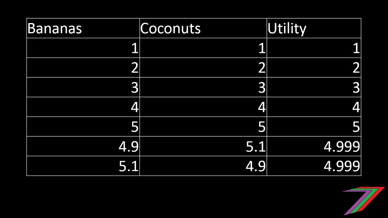
Robinson Crusoe is stranded on an island. This island has only 2 natural resources, bananas and coconuts. Robinson Crusoe needs both bananas and coconuts to survive. Robinson Crusoe’s survival can be observed using a Cobb-Douglas utility function (multiplicative utility function). If Robinson Crusoe has either no coconuts or bananas, his utility will be zero (will die). His utility function will look something like the following equation.
Utility = Coconut^(1/2) × Banana^(1/2)
For more information on utility, you can access my utility post using the following link: https://steemit.com/economics/@spectrumecons/economic-concepts-1-utility
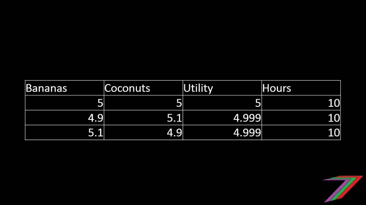
For simplicity, I have assumed that Robinson Crusoe likes bananas and coconuts equally. Robinson Crusoe’s preference would be to have an equal proportion of bananas and coconuts. The tables below show the amount of utility Robinson Crusoe can obtain from different combinations of bananas and coconuts.
We can also prove mathematically using differential calculus that Robinson Crusoe obtains the most utility from consuming equal amounts of bananas and coconuts. For those interested, the proof is in the following equations.
δUtility/δCoconut = ½ × Banana(1/2)/Coconut(1/2) = 0
δUtility/δBanana = ½ × Coconut(1/2)/Banana(1/2) = 0
Banana(1/2)/Coconut(1/2) = Coconut(1/2)/Banana(1/2)
Banana = Coconut
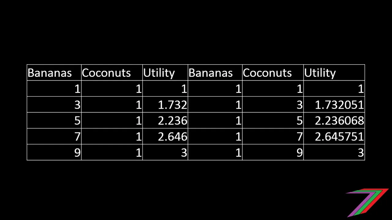
Bananas and coconuts do not magically appear. Robinson Crusoe needs to gather or pick them. Therefore, Robinson Crusoe also has a production function. Robinson Crusoe also does not have unlimited time to collect bananas and coconuts in a day. Robinson Crusoe only has 10 hours he can spare for collecting food; this is Robinson Crusoe’s constraint. Robinson Crusoe takes 2 hours to pick a coconut and 1 hour to pick a banana. Robinson Crusoe’s production function and constraint can be expressed as follows:
2 × Coconut + Banana = 10
Since collecting coconuts requires twice as much time and effort as picking bananas. Robinson Crusoe gathers twice as many bananas as coconuts. I can demonstrate this using the tables below.
We can also prove mathematically using differential calculus that Robinson Crusoe obtains the most utility from gathering and consuming twice as many bananas as coconuts. For those interested, the proof is in the following equations.
Utility function – Production Function Constraint
Utility = Coconut^(1/2) × Banana^(1/2) – (2 × Coconut + Banana – 10)
δUtility/δCoconut = ½ × Banana(1/2)/Coconut(1/2) - 2 = 0
δUtility/δBanana = ½ × Coconut(1/2)/Banana(1/2) - 1 = 0
Banana(1/2)/Coconut(1/2)/Coconut(1/2)/Banana(1/2) = 2
Banana(1/2)/Coconut(1/2) = 2 × (Coconut(1/2)/Banana(1/2))
Banana = 2 × Coconut
Substitute “Banana = 2 × Coconut” into the production function constraint
4 × Coconut = 10
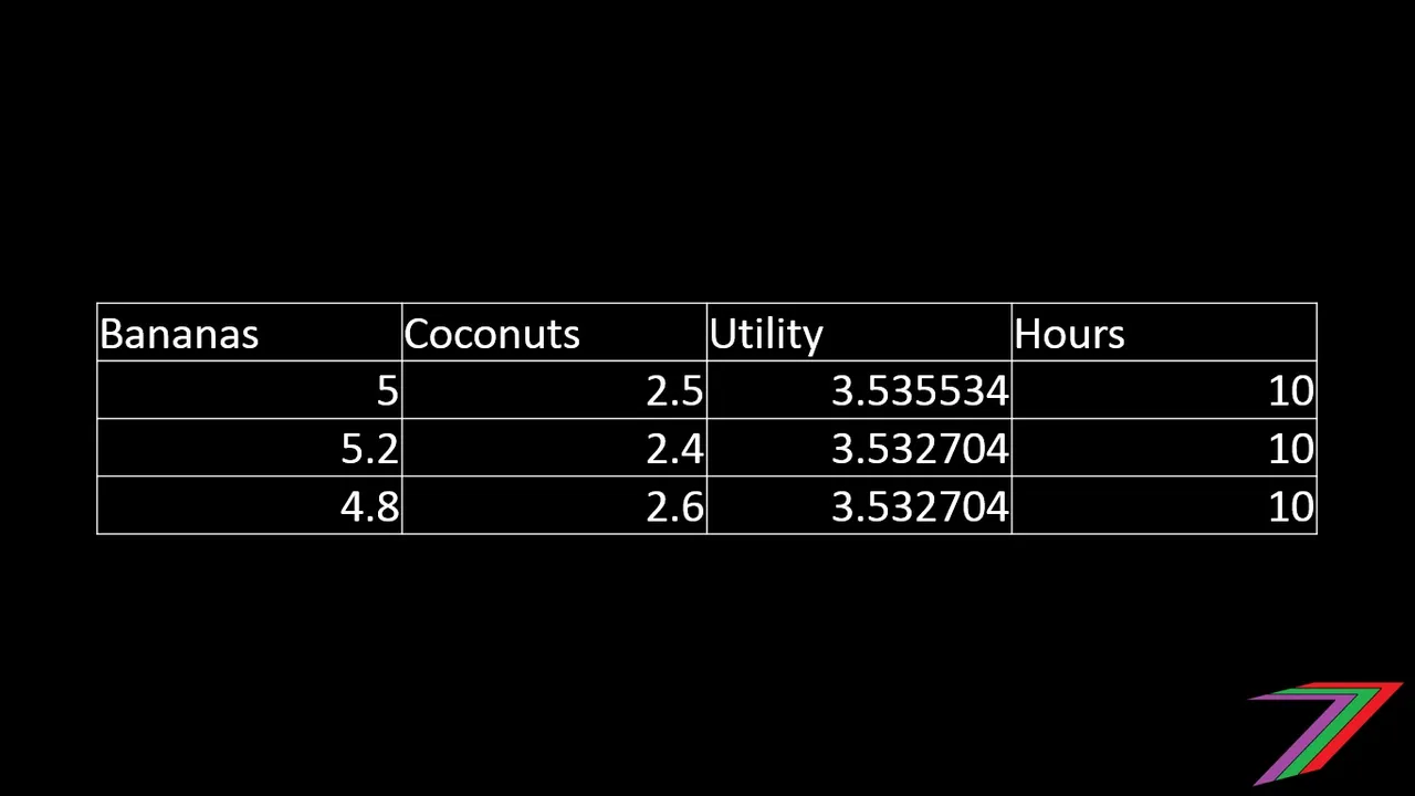
Coconut = 2 ½ (It sounds silly gathering 2 ½ coconuts a day, to make it feel more realistic imagine that he gathers 5 coconuts over a two day period)
Substitute “Coconut = 2 ½” into the production function constraint
2 × 2 1/2 + Banana = 10
Banana = 5
Substitute “Banana = 5” and “Coconut = 2 ½” into the utility function.
Utility = 2 ½^1/2 × 5^1/2 = 3.535534
What if Robinson Crusoe discovered a new method of collecting coconuts that allowed him to be able to take one hour instead of two hours to collect a coconut? Robinson Crusoe would now have a different production function constraint. The new production function constraint would look as follows:
Coconut + Banana = 10
Now that collecting coconuts and bananas require the same amount of time and effort and Robinson Crusoe also gains the same level of utility from both. Robinson Crusoe will now gather the same number of coconuts as bananas. I can demonstrate this using the tables below.
We can also prove mathematically using differential calculus that Robinson Crusoe obtains the most utility from gathering and consuming the same number of bananas as coconuts. For those interested, the proof is in the following equations.
Utility function – Production Function Constraint
Utility = Coconut^(1/2) × Banana^(1/2) – (Coconut + Banana – 10)
δUtility/δCoconut = ½ × Banana(1/2)/Coconut(1/2) - 1 = 0
δUtility/δBanana = ½ × Coconut(1/2)/Banana(1/2) - 1 = 0
Banana(1/2)/Coconut(1/2)/Coconut(1/2)/Banana(1/2) = 1
Banana(1/2)/Coconut(1/2) = Coconut(1/2)/Banana(1/2)
Banana = Coconut
Substitute “Banana = Coconut” into the production function constraint
2 × Coconut = 10
Coconut = 5
Substitute “Coconut = 5” into the production function constraint
5 + Banana = 10
Banana = 5
Substitute “Banana = 5” and “Coconut = 5” into the utility function.
Utility = 5^1/2 × 5^1/2 = 5
Implications from the Robinson Crusoe Model
In our Robinson Crusoe example, we analysed the impact of an improvement in collecting coconuts. In the real world this could be equivalent to the discovery of an amazing new technology that allows the doubling of a particular output. As a result of the improvement in collecting coconuts, Robinson Crusoe can collect an additional 2 ½ coconuts a day (change in output). Robinson Crusoe also increases his level of utility (happiness/satisfaction) from 3.535534 Utils to 5 Utils (A Util is a measure for Utility). Robinson Crusoe still allocates 5 hours to gathering coconuts and 5 hours to picking bananas (unchanged usage of resources).
What has been excluded from the Robinson Crusoe example that I provided is the level of satisfaction Robinson Crusoe gets from picking bananas and collecting coconuts and the possible reduction in hours of work. Robinson could spend more time picking bananas because picking bananas is really fun, while collecting coconuts is really boring. The additional productivity gains from improved coconut collecting might tempt Robinson Crusoe to work 8 hours instead of 10 hours. These factors can be included in the Robinson Crusoe Model but it will make the calculations rather tedious for this post. Still, I hope you get the general idea.
The impact of Robinson Crusoe’s improved ability to collect coconuts can also be represented using indifference curves (these are curves that represents constant values of utility) and production possibility frontiers (combinations of optimal levels of production, producing on this frontier can be considered productively efficient). The indifference curves and production possibility frontiers in figure below demonstrates Robinson Crusoe’s increased productive from improved coconut collecting as well as the additional utility he obtains from shifting to another indifference curve. I will be covering indifference curves and production possibility frontiers in another post.
Production Possibility Frontiers and Indifference Curves for Robinson Crusoe Model
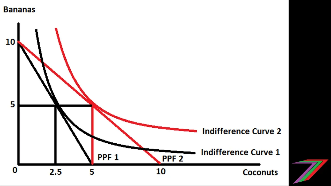
Where:
Indifference Curve 1 = 3.535534
Indifference Curve 2 = 5
Basic Input-Output Model
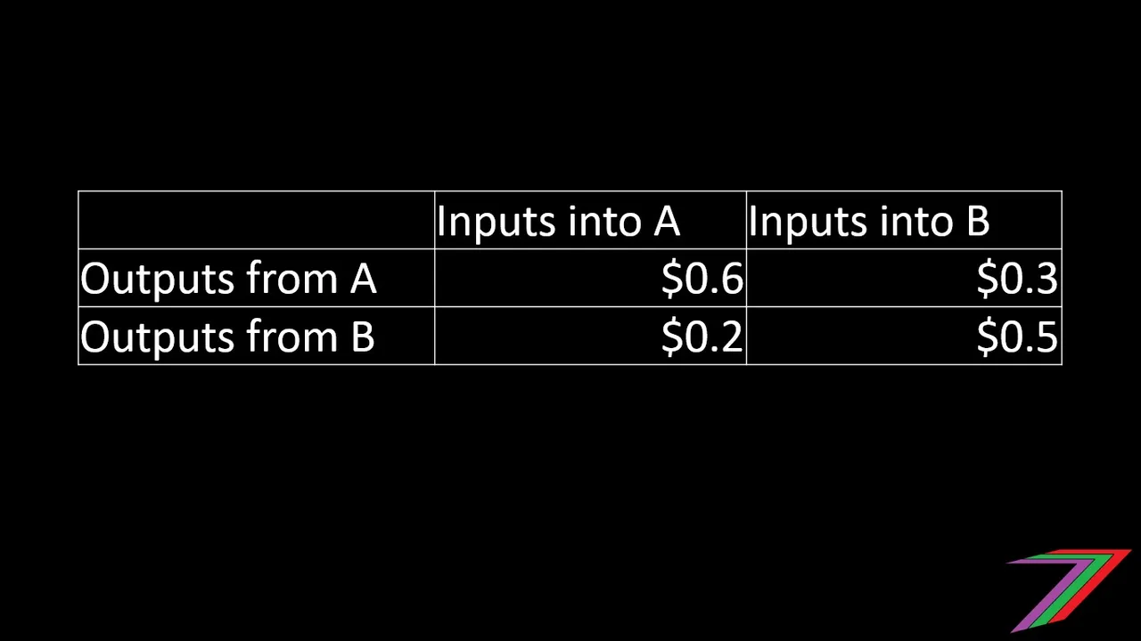
General Equilibrium can also be partly explained using Input-Output Models. I thought I would briefly explain general equilibrium using the Input-Output Model approach. Let’s imagine that there are only two industries in the world. They are industry A and Industry B. Firms in Industries A and B receive inputs from each other to produce a final output for consumption.
For every dollar of goods sold from Industry A, there is an input cost of $0.6 from firms within Industry A and an input cost of $0.2 from firms within Industry B. For every dollar of goods sold from Industry B, there is an input cost of $0.5 from firms within Industry B and an input cost of $0.3 from firms within Industry A.
What if sales increase by $1 for either Industries A or B?
Let’s start with Industry A. Output of Industry A increases directly by $1 from increased consumption. Output of Industry A also increases by $0.6 as a direct input into the production in Industry A. Output of Industry B increases by $0.32 (1.6 × 0.2) for the direct production of the additional $1.6 output from Industry A. Output from Industry A is required to increase further as Industry A provides input into Industry B. This creates a multiplier effect on the output for both industries A and B. The same happens if the output from Industry B increases by $1 from consumption.
The table below provides a rough calculation of the overall increase in output for both Industries A and B. The table shows calculations over several rounds of the two industries providing inputs to each other until the required input is close to zero.
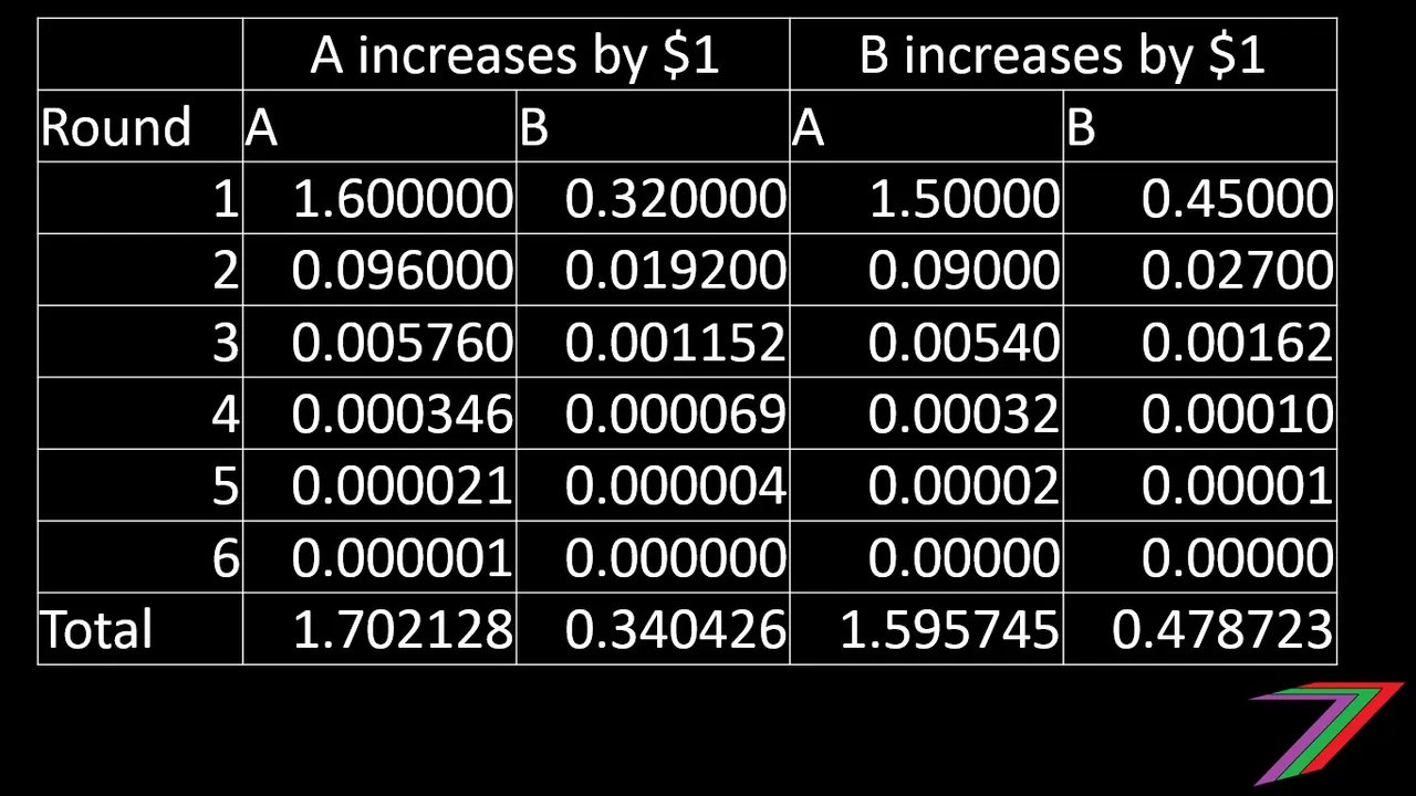
The total value of output produced from a $1 increase in direct output from consumption is shown in the table below.
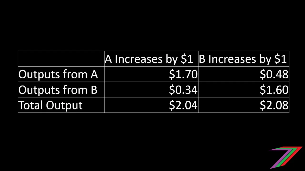
The most important point to grasp from this simple example is that there is a flow on effect from increases in demand from just one industry that can flow across multiple industries thus generating larger changes in total output than just the initial increase.
It is also interesting to note that a direct $1 increase in consumption of Industry B's output produces a larger flow on effect than a direct $1 increase in consumption of Industry A's output. This is because of the larger input requirement of Industry A into Industry B than vice versa.
Conclusion
This brings me to the end of this very technical post. I hope I have not lost too many of you today with all the mathematics and economic theory. General Equilibrium Theory attempts to explain how changes in one area can have flow on effects to many other areas. We should not look at anything in isolation as most things are connected in one way or another even if those linkages can sometimes be very indirect. It is important to have a grasp of the implications of General Equilibrium Theory but it is not necessary to fully understand all the technical aspects of it.

The CGE and Input-Output Models are used to apply General Equilibrium Theory to the real world. These models attempt to quantify the relationships between various industries and sectors within the economy. The cost and time that goes into running these models often makes them impractical for economic impact analysis.
Cost Benefit Analysis is far less costly and time consuming than CGE or Input-Output Modelling. Cost Benefit Analysis can provide sufficient information to decision-makers regarding the viability of many policies and initiatives. I have not discussed Cost Benefit Analysis in this post but I have several other posts that explain how a Cost Benefit Analysis can be done. Here is the link to my first Steemit post which contains a video that explains Cost Benefit Analysis in some detail: https://steemit.com/economics/@spectrumecons/cost-benefit-analysis-video
Thank you for spending the time to read this post. I have many more economic concept posts to come. Most of these posts will not be as technical as this post.