As said in my last weekly particle physics blog, last week was at the same time very emotional and very busy work-wise, so that I did not find the time to write the present post before today. There is however some good in this situation, as it gave more time to a few to embark into our joint citizen science adventure on Hive. On second thought, I may consider writing one of these blogs every other week. I will take a decision depending on how fast the reports originating from the present blog will appear, and on any potential feedback on this matter.
The previous episode was dedicated to the installation of a piece of software that will be heavily used within this citizen particle physics project. I recall that the project requires the simulation of a signal of physics beyond the Standard Model (related to neutrino physics), and how to assess it in future data at CERN’s Large Hadron Collider (from the overwhelming background of the Standard Model). Those simulations will be achieved with this installed software.
I was amazed by the level of engagement and participation following the first post on this project. I had the chance to read (so far, as it is never too late to join us) seven reports from the participants, from agreste, eniolw, gentleshaid (please let us know whether all your problems have been sorted out), mengene, metabs, servelle and travelingmercies. Following our particle physics standards, the author list is alphabetically ordered. I would nevertheless like to single out the work done by @metabs, whose report consists of a comprehensive review on how to get started on a Windows system via a virtual machine.
The goal of the present blog is to allow everyone to become expert users of the MG5aMC software, or at least users that are expert enough to deal with all simulations to be performed during the project. As promised at the end of the previous episode, this post is based on the tutorial shipped with MG5aMC. It however goes independently of it, so that I could explain the physics that comes with it on a step-by-step basis.
Before starting, I acknowledge in advance all potential participants and interested supporters from our community: @agmoore, @agreste, @aiovo, @alexanderalexis, @amestyj, @darlingtonoperez, @eniolw, @firstborn.pob, @gentleshaid, @isnochys, @ivarbjorn, @mengene, @mintrawa, @servelle, @travelingmercies and @yaziris. Feel free to let me know if you want to be added or removed from this list.

[Credits: geralt (Pixabay)]
Top-antitop production at the LHC - task 1
In order to get used to MG5aMC properly, we will simulate collisions such as those ongoing at CERN’s Large Hadron Collider. In each of those collisions, a pair of top quarks (actually, one top quark and one antitop quark) is produced.
Among all particles of the Standard Model of particle physics, the top quark is the heaviest. It can be seen as a heavy big brother of the up quark, one of the elementary particles giving rise to protons and neutrons. For more information, please consider having a look to this blog on the Standard Model and this one in which some information on the top quark is provided. By virtue of its large mass, the top quark is considered as a perfect portal to new particle physics phenomena, and its properties are therefore under deep scrutiny experimentally (to verify whether there is no hint of an anomaly).
Let me now introduce the first task. The MG5aMC code can be started as indicated in the previous episode. I recall that this requires to open a shell, and move to the folder in which MG5aMC has been unpacked (MG5_aMC_v2_9_9 in my case). Then the code is started by typing in the shell:
cd MG5_aMC_v2_9_9;
./bin/mg5_aMC
If everything goes well, you should have a prompt MG5aMC> that is waiting for instructions. We are ready to define the process considered within the code. By checking the screen output we can observe the following
Multiparticle labels:
p = g u c d s u~ c~ d~ s~
j = g u c d s u~ c~ d~ s~
l+ = e+ mu+
l- = e- mu-
vl = ve vm vt
vl~ = ve~ vm~ vt~
all = g u c d s u~ c~ d~ s~ a ve vm vt e- mu- ve~ vm~ vt~ e+ mu+ t b t~ b~ z w+ h w- ta- ta+
The last line is very useful as it indicates all particles that are available within the model of physics (that is by default the Standard Model). We can note the presence of t (a top quark) and t~ (a top antiquark). In addition, the first of the above line defines the elementary particle content of the proton. We can see that it is composed of many quarks and antiquarks, as well as of gluons.
At high energies, a proton is an object made of interacting quarks and antiquarks (the most elementary building blocks of matter and the associated antiparticles) and gluons (the mediators of the strong force). To get more information on this, I refer to the second section of this blog on particle collider simulations.
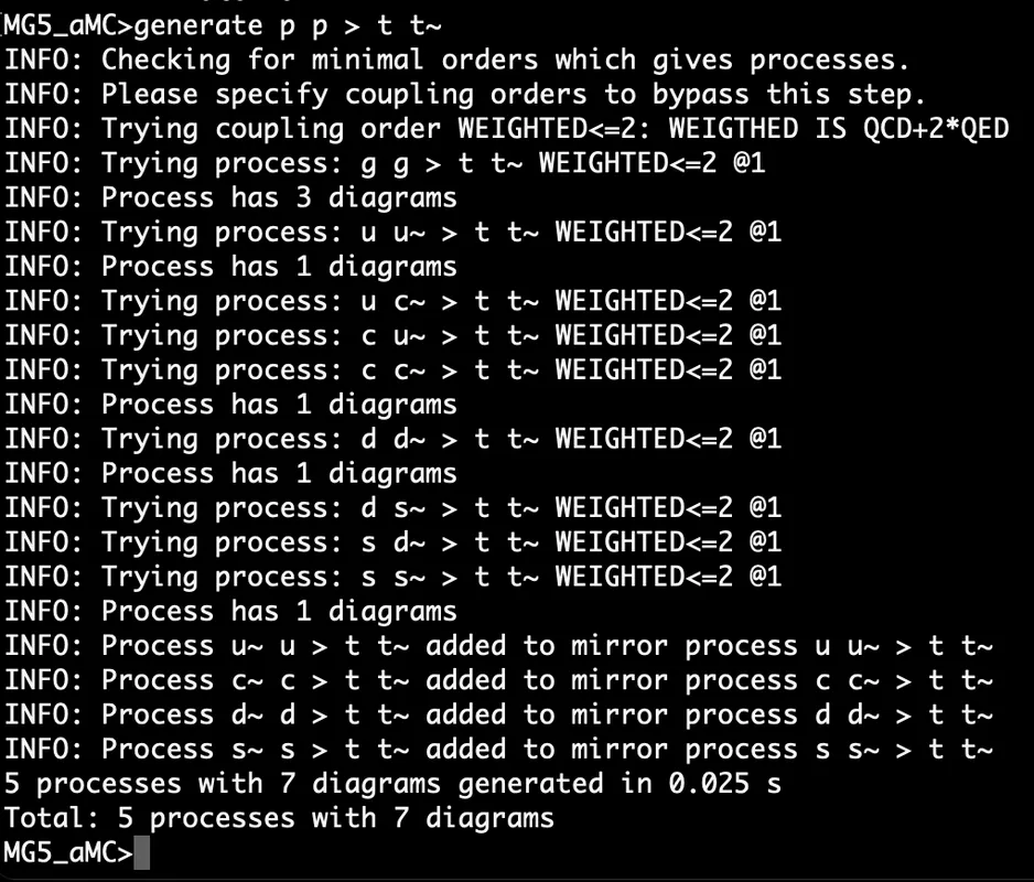
We thus have all the information necessary to define the collider process of interest, the production of a top-antitop pair in proton-proton collisions. This definition is performed by typing in the MG5aMC command line interface
generate p p > t t~
The syntax is in principle self-explanatory at this stage. > stands for an arrow. The initial state of the process (two protons) is put on its left, each particle being separated by a space. This gives p p as we consider proton-proton collisions. The final state of the process is put on the right of the arrow, each particle being again separated by a space. This gives t t~ as we produce one top quark and one antiquark. The resulting screen output gives:
[Credits: @lemouth]
This command makes the code ready to deal with the quantum field theory calculation associated with the process of interest. It relies on Feynman diagrams, that embed all possibilities to connect the initial state of the process to its final state. For more details, please check out the second section of this blog. Diagrams can be displayed by typing in
display diagrams
I recommend to type this command to see that we have many options to produce a top-antitop pair at colliders such as the LHC, from different initial states (any combination formed from the constituents of the two proton would work).
A Fortran code for top-antitop production at the LHC - task 2
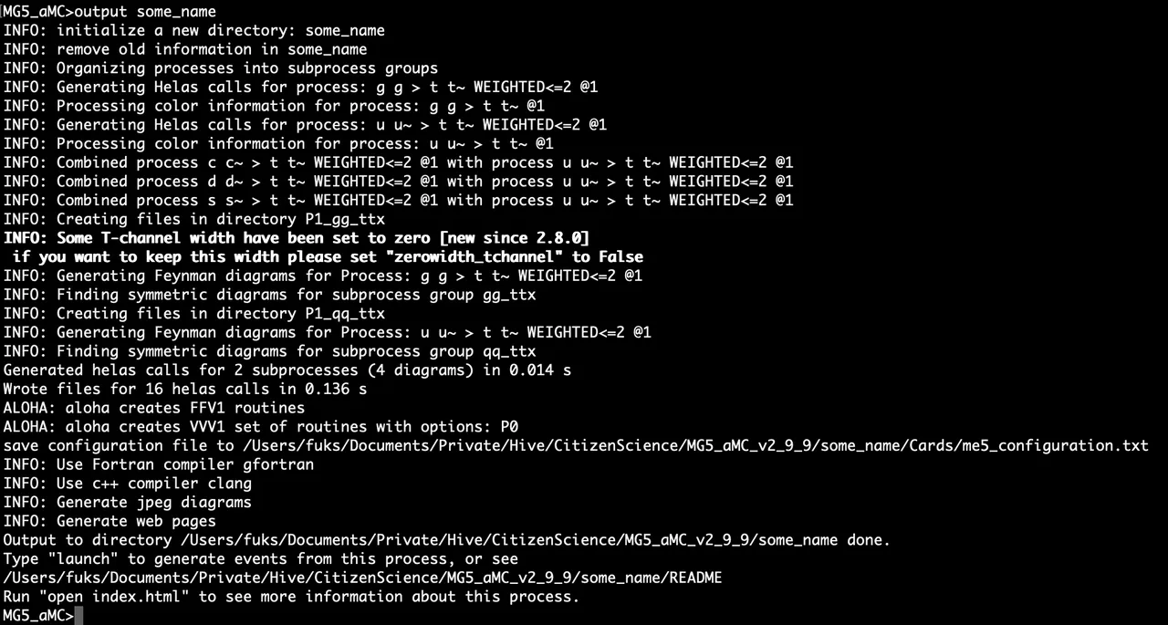
Now, it is time to instruct the code to extract an equation from these diagrams (a heavy integral) and convert it to a Fortran code. From this equation, it will then become possible to simulate collisions as they would occur in nature. For details, I once again refer to this older blog. The code is obtained by typing in
output some_name
In this command, some_name can be replaced by your favourite name, and corresponds to the folder in which the results will be stored. This gives:
[Credits: @lemouth]
We next quit MG5aMC by typing
exit
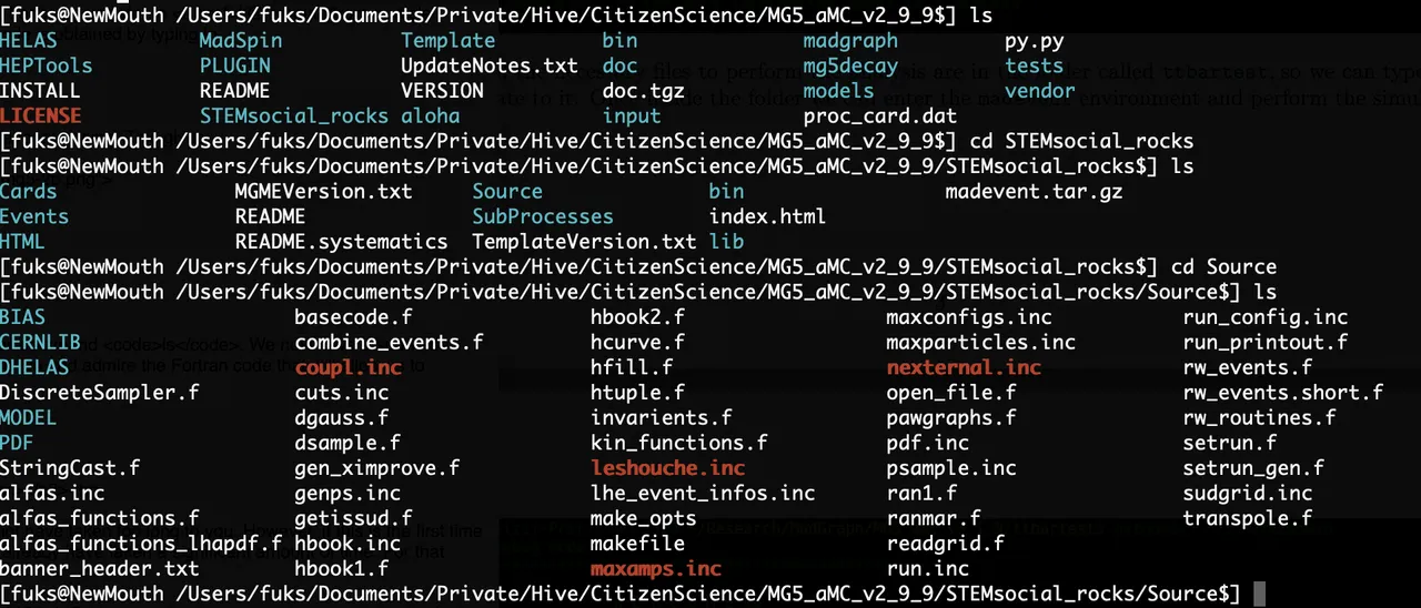
The following item on our to-do list is to list the content of the current folder (through the Linux command ls). We see a sub-folder named some_name. You can check out its content for the fun and admire the Fortran code that will allow us to simulate LHC collisions leading to the production of a top-antitop pair.
In practice, you can try to mimic what I did in the screenshot below. Feel free to open any file with a text editor if you are curious ;)
[Credits: @lemouth]
Computing the rate to top-antitop production at the LHC - task 3
Having a Fortran code dedicated to a given calculation is great. Compiling it and running it is better. These tasks are highly automated and there is not much to do on your side. Please go back to the folder in which MG5aMC has been installed, and restart the code as mentioned above. Then type
launch some_name
That’s all! MG5aMC will compile the code, execute it and produce the output. For this week we are not interested in understanding how to interpret the results. The goal is instead to solely produce them, and verify whether everything runs smoothly without any problem.
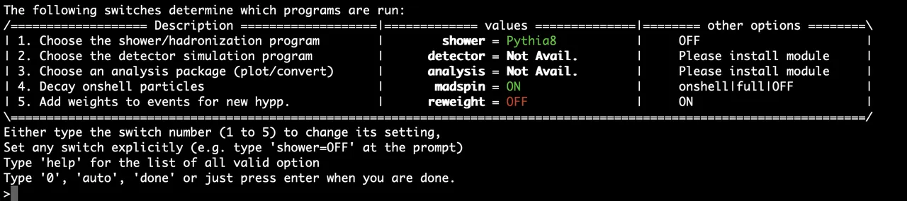
As an outcome of the launch command, there is an interactive menu allowing us to discuss with MG5aMC. We need to tell it to use Pythia8 and MadSpin (for which f2py, that is part of NumPy, should be present on the system; if this is not the case, please proceed with its installation). This is achieved as follows.
- To enable Pythia8, press 1 (then press enter).
- To enable MadSpin, press 4 (then press enter).
We should then get something like this:
[Credits: @lemouth]
Pythia8 allows us to simulate the strongly-interacting environment of the LHC. This includes parton showering (radiation of strongly-interacting particles by other strongly-interacting particles) and hadronisation (formation of composite objects made of quarks and gluons). For more information, feel free to check out this blog. On the other hand, MadSpin deals with the decay of the produced top quarks, that are instable particles (see here).
The next step is to set the simulation parameters. First press enter so that a new menu is displayed.
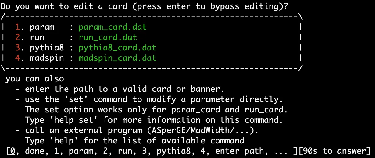
[Credits: @lemouth]
We have four cards to play with.
- The
param_cardallows us to change the parameters of the particle physics model. - The
run_cardallows us to change the collider settings. - The
pythia8_cardallows us to change the parameters of Pythia8. - The
madspin_cardallows us to modify how heavy instable particles decay.
Let’s keep everything as default for now, with one exception. We open the run_card (by pressing 2 and the enter), and then go to line 129. This line should read
True = use_syst ! Enable systematics studies
and needs to be changed into
False = use_syst ! Enable systematics studies
In order to do it, MG5aMC should in principle detect a text editor coming with your machine and open the file with it. In my case it is VIM, so that it is sufficient to type
129 G d d i
and then edit the line. Finally, the file can be saved by typing
:wq
If you don’t do that, please don’t worry. The code should just crash because some packages are missing… So please do it ;)
Then, it is sufficient to press enter. The simulation starts and will produce some long output printed to the screen. Please check it out. In the middle of it, you should see something similar to
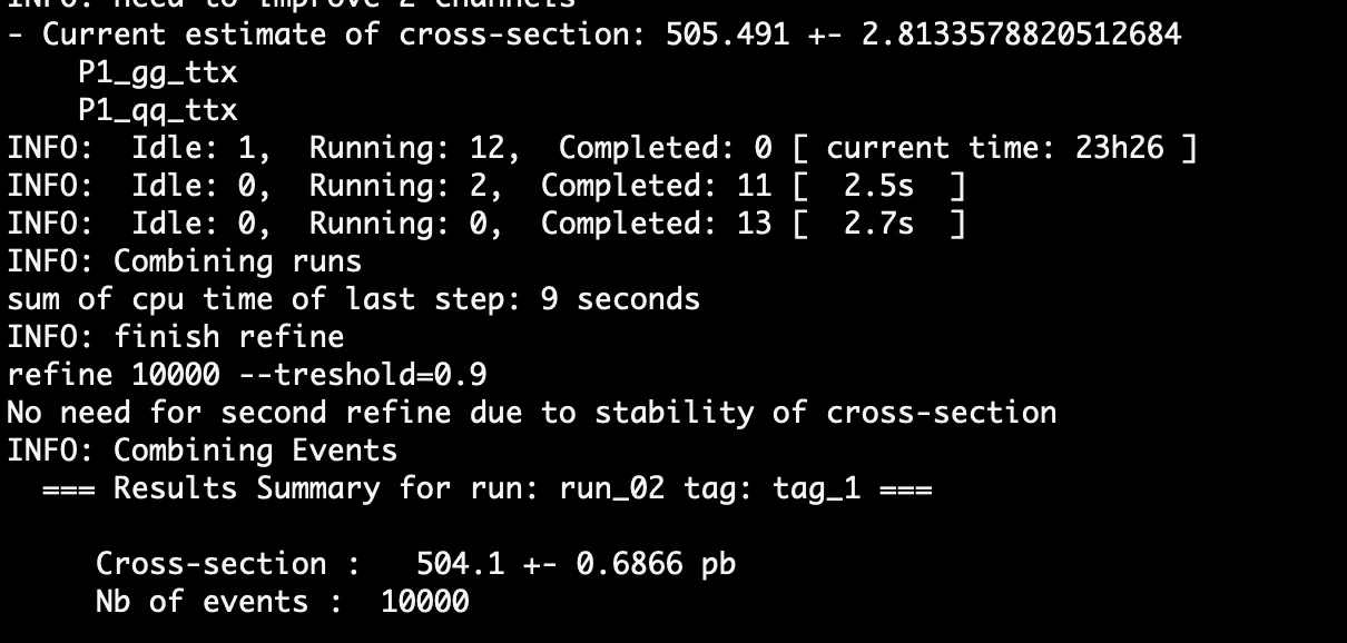
[Credits: @lemouth]
This number (505.491 ± 0.6866 pb) corresponds to the production rate of a top-antitop pair at the LHC. The result that you will obtain could be slightly different from mine. The reason is that MG5aMC achieve a Monte Carlo simulation based on some random scan. Small numerical discrepancies are possible, although the numbers should be compatible within their uncertainties (here we have a per-mille level precision).
In the performed calculations, we kept all default values in the run_card, so that 10,000 collisions have been simulated. With a larger number, a larger precision is automatically obtained.
The units of the rate may be strange to you. Those consist of picobarns (abbreviated to pb). In order to understand what they mean, we can invoke the amount of recorded LHC data: 140/fb. This number is given in inverse femtobarns. 1 inverse femtobarn is equal to 1,000 inverse picobarns, so that the amount of recorded LHC data reads 140,000/pb. Multiplying the calculated rate in pb by 140,000/pb, we obtain a dimensionless quantity of about 70,000,000. This consists of the amount of top-antitop events excepted in current data.
MG5aMC thus calculates the rate of any given process, and we can extract from this information the amount of collisions that should be recorded and related to the process considered. This is thus a very useful quantity!
Checking out whether everything went fine - task 4
In the rest of the screen output, we can verify that MadSpin handled the decay of the produced top quarks and antiquarks as expected. Please verify that you see something like this on your screen.
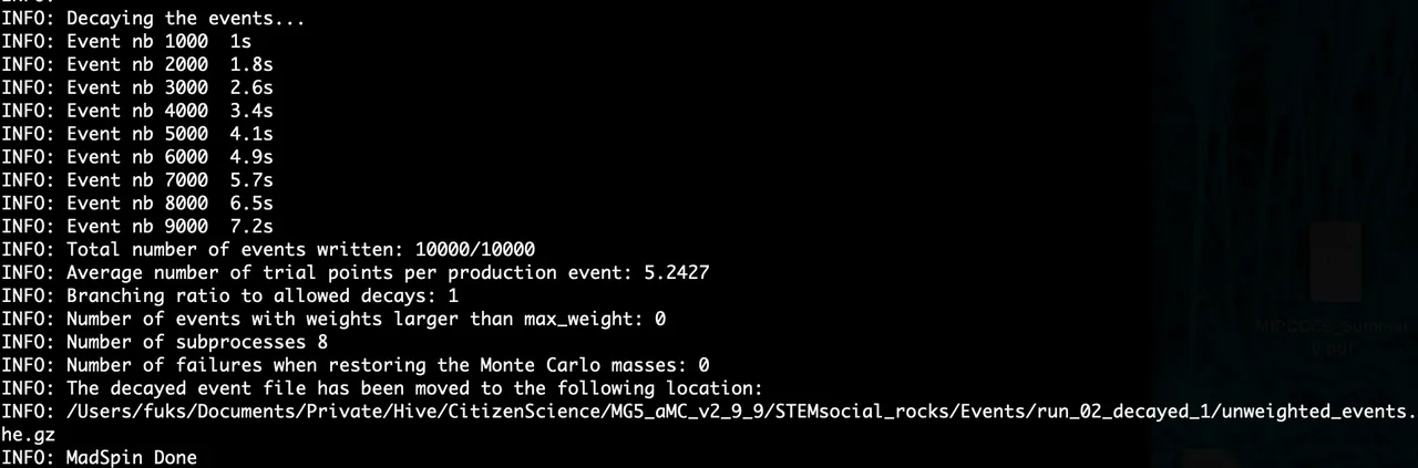
[Credits: @lemouth]
Similarly, we can verify that parton showering and hadronisation went fine:
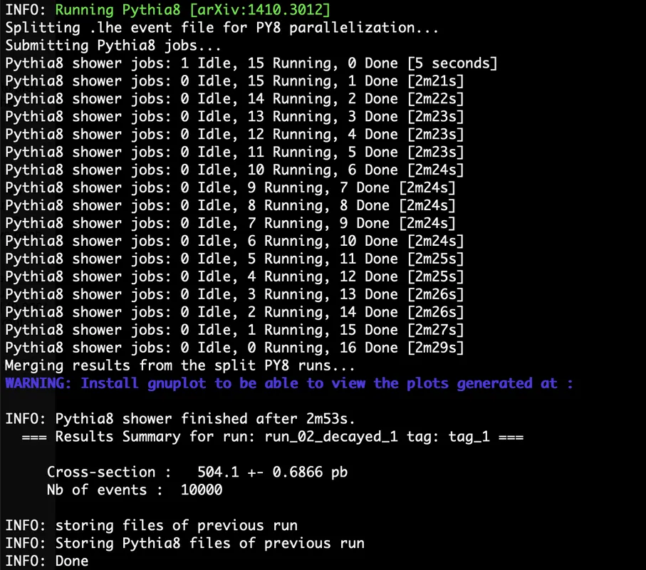
[Credits: @lemouth]
We now have on our disk a file containing 10,000 LHC collisions in which a top-antitop pair has been produced. By exiting the code (through typing exit), we can verify that those events are well available on disk.
cd some_name/Events/run_01_decayed_1
ls -lrt
We should have here a file if about 800 MB named tag_1_pythia8_events.hepmc.gz. This is the file we will analyse to understand the physics that is in there. But this will be for the next episode. Reaching this stage is enough for this week.
Summary: mastering particle collider simulations
Two weeks ago, we spent time on the installation of a program named MG5aMC. In the blog of this week, I proposed a few tasks to get used to this program. This is an incontrovertible prerequisite before being able to fully work on our citizen science particle physics project on Hive.
I proposed here something very simple: the simulation of 10,000 proton-proton collisions such as those happening in the Large Hadron Collider. In those collisions, a top quark and an antitop quark are produced.
Those simulated collisions were quite accurate in the sense that they include the core process considered, the decay of the top and antitop quarks, parton showering and hadronisation. Somewhat, they are as close as possible as what is going on in true collisions. The missing steps concern the simulation of the detector, and the reconstruction of the obtained events. A collision indeed generally leads to thousands of produced particles. However, these correspond only to a handful of higher-level objects that can be reconstructed and used in an analysis.
As usual, I warmly welcome everyone interested to try out the tasks proposed this week. I am here to help, answer questions and solve problems. If you are new to this and interested in joining us, please check the previous blogs on the topic (here and there), as well as the reports available from the #citizenscience tag.
If you are a participant to the project, I am looking forward to read a blog detailing your progress. Please make sure to notify me and use the #citizenscience tag.
Have a nice week, full of particle physics!